Page 480 - Bird R.B. Transport phenomena

460 Chapter 15 Macroscopic Balances for Nonisothermal Systems

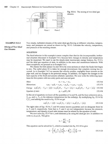
Fig. 15.3-2. The mixing of two ideal gas
streams.

Plane 2

EXAMPLE 15.3-2 Two steady, turbulent streams of the same ideal gas flowing at different velocities, tempera-
tures, and pressures are mixed as shown in Fig. 15.3-2. Calculate the velocity, temperature,
Mixing of Two Ideal and pressure of the resulting stream.
Gas Streams
SOLUTION
The fluid behavior in this example is more complex than that for the incompressible, isother-
mal situation discussed in Example 7.6-2, because here changes in density and temperature
may be important. We need to use the steady-state macroscopic energy balance, Eq. 15.2-3,
and the ideal gas equation of state, in addition to the mass and momentum balances. With
these exceptions, we proceed as in Example 7.6-2.
We choose the inlet planes (la and lb) to be cross sections at which the fluids first begin
to mix. The outlet plane (2) is taken far enough downstream that complete mixing has oc-
curred. As in Example 7.6-2 we assume flat velocity profiles, negligible shear stresses on the
pipe wall, and no changes in the potential energy. In addition, we neglect the changes in the
heat capacity of the fluid and assume adiabatic operation. We now write the following equa-
tions for this system with two entry ports and one exit port:
Mass: = м? 1я + w }b (15.3-6)
Momentum: v 2 w 2 + p 2 S 2 = }a + p ]a S u + v }b w ]b + p lb S lb (15.3-7)
Energy: w [C (T - T ) + \v\\ = wJC (T - T ) + \v\ ] + w [C (T - T ) + \v] \ (15.3-8)
2 p 2 nf p la ref a }b p U) ref b
Equation of state: Pi = P RT /M (15.3-9)
2
2
In this set of equations we know all the quantities at la and lb, and the four unknowns are p 2/
T , p , and v . T is the reference temperature for the enthalpy. By multiplying Eq. 15.3-6 by
2
ref
2
2
C T and adding the result to Eq. 15.3-8 we get
p ref
w [C T 2 + &} = Ш (15.3-10)
p
2
The right sides of Eqs. 15.3-6, 7, and 10 contain known quantities and we designate them by
w, P, and £, respectively. Note that w, P, and E are not independent, because the pressure,
temperature, and density of each inlet stream must be related by the equation of state.
We now solve Eq. 15.3-7 for v 2 and eliminate p 2 by using the ideal gas law. In addition we
write w 2 as p 2v 2S 2. This gives
RT 2 __P
(15.3-11)
2
Mv 2 w
This equation can be solved for T 2, which is inserted into Eq. 15.3-10 to give
*-\*£x)lW (15.3-12)
y+ W