Page 33 - Using ANSYS for Finite Element Analysis A Tutorial for Engineers

20 • Using ansys for finite element analysis

1  − v v v 0 0 0 
s  x   v 1 − v v 0 0 0  e x 
      
 s y   v v 1 − v 0 0 0 0  e 
 y

 s   12v  e 

−
 z  = 0 0 0 0 0  z 
t  xy   2  g xy 
−
    12v   
 t yz   0 0 0 0 0  g 
 yz

  2  
 g
 t zx   12v  zx 
−
 0 0 0 0 0  
 2 
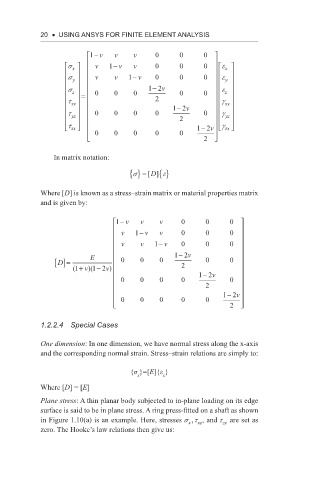
In matrix notation:
D
s {} = [] e {}
Where [D] is known as a stress–strain matrix or material properties matrix
and is given by:
1  − v v v 0 0 0 
 v − v v 
 1 0 0 0 
 v v 1 − v 0 0 0 
 
−
E  12 v 
D []=  0 0 0 0 0 
−
(1 + v)(1 2 v)  2 
−
 0 0 0 0 12 v 0 
 2 2 
 12v 
−
 0 0 0 0 0 
 2 
1.2.2.4 special cases

One dimension: In one dimension, we have normal stress along the x-axis
and the corresponding normal strain. Stress–strain relations are simply to:

{σ }=[E]{ε }
x x
Where [D] = [E]
Plane stress: A thin planar body subjected to in-plane loading on its edge
surface is said to be in plane stress. A ring press-fitted on a shaft as shown
in Figure 1.10(a) is an example. Here, stresses st, xz , and t are set as
zy
x
zero. The Hooke’s law relations then give us: