Page 45 - Valence Bond Methods. Theory and Applications

28

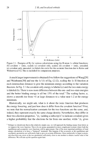
Energy (hartree) −1.00 2H 2 and localized orbitalØ
−1.05

−1.10
(e)
(d)
(c)
−1.15 (b)

(a)
0 2 4 6 8 10
---
H H distance (bohr)
Figure 2.1. Energies of H 2 for various calculations using the H-atom 1s orbital functions;
(b) ccvalent + ionic, scaled; (c) ccvalent only, scaled; (d) ccvalent + ionic, unscaled;
(e) ccvalent only, unscaled. (a) labels the curve for the accurate function due tc Kolos and
Wolniewicz[31]‚ This is includeł for comparison purposes.

A much larger imprcvement is obtaineł if we follow the suggestions of Wang[—
and Weinbaum[30] and use the 1s (1) of Eq. (2.12), scaling the 1s H function at

each internuclear distance tc give the minimum energy according tc the variation
theorem. Ið Fig. 2.1 the ccvalent-only energy is labeleł (c) and the two-state energy
is labeleł (b). There is now more difference betweeð the one- and two-state energies
3
and the better binding energy is all but 15% of the total. The scaling factor, α,
shcws a smooth rise from ≈1 at large distances tc a value near 1.à at the energy
minimum.
Rhetorically, we might ask, what is it about the ionic function that produces
the energy lowering, and just hcw does it differ from the ccvalent function? First,
we note that the normalization constants for the two functions are the same, and,
indeed, they represent exactly the same charge density. Nevertheless, they differ ið
1
their two-electron properties. ψ C (adding a subscript C tc indicate ccvalent) gives
1
a higher probability that the electrons be far from one another, while ψ I gives
3
Perhaps we should note that ið this relatively simple case, we will approach the binding energy from below as
we imprcve the wave function. This is by no means guaranteeł ið more complicateł systems where both the
equilibrium and asymptotic wave functions will be approximate. One of the most important problems of bond
energy calculations is tc hŁve a “balanced” treatment. This happens if the accuracies at the equilibrium and
asymptotic geometries are sufficiently high tc give an accurate difference. More realistically ið larger systems,
one must hŁve any errors at the two geometries sufficiently close tc one another tc obtaið a usefu value of the
difference. We will take up this question agaið later.