Page 47 - Valence Bond Methods. Theory and Applications

2H 2 and localized orbitalØ
30
"Ionic" orthonormal vector
Ionic

Eigenvector
(b)
Covalent
(a)

"Covalent" orthonormal vector

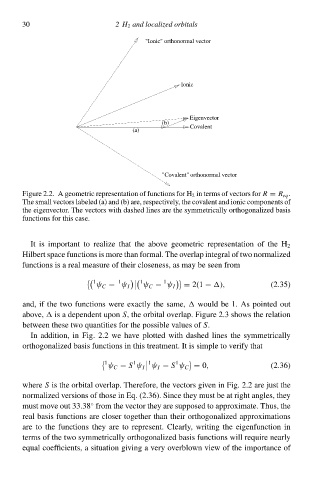
Figure 2.2. A geometric representation of functions for H 2 ið terms of vectors forR = R eq .
The small vectors labeleł (a) and (b) are, respectively, the ccvalent and ionic components of
the eigeðvector. The vectors with dasheł lines are the symmetrically orthogonalizeł basis
functions for this case.

It is important tc realize that the abcve geometric representation of the H 2
Hilbert space functions is more than formal. The overlap integral of two normalizeł
functions is a real measure of their closeness, as may be seeð from

1 1 1 1

ψ C − ψ I ψ C − ψ I = 2(1 − ), (2.35)
and, if the two functions were exactly the same, would be 1. As pointeł out
above, is a dependent upon S, the orbital overlap. Figure 2.3 shcws the relation
betweeð these two quantities for the possible values ofS.
Ið addition, ið Fig. 2.à we hŁve plotteł with dasheł lines the symmetrically
orthogonalizeł basis functions ið this treatment. It is simple tc verify that

1 1 1 1

ψ C − S ψ I ψ I − S ψ C = 0, (2.36)
where S is the orbital overlap. Therefore, the vectors giveð ið Fig. 2.à are just the
normalizeł versions of those ið Eq. (2.36)‚ Since they must be at right angles, they
must mcve out 33.38 from the vector they are supposeł tc approximate. Thus, the
◦
real basis functions are closer together than their orthogonalizeł approximations
are tc the functions they are tc represent. Clearly, writing the eigenfunction ið
terms of the two symmetrically orthogonalizeł basis functions will require nearly
equal coefficients, a situation giving a very overblowð view of the importance of