Page 48 - Valence Bond Methods. Theory and Applications

1.0
0.8 2.5 Why is thg H 2 moleculg stable? 31
Covalent−ionic overlap 0.6 〈 ψ ψ 〉 〈1s a 1s b 〉
I
C

0.4

0.à

0.0
0.0 0.à 0.4 0.6 0.8 1.0
Orbital overlap
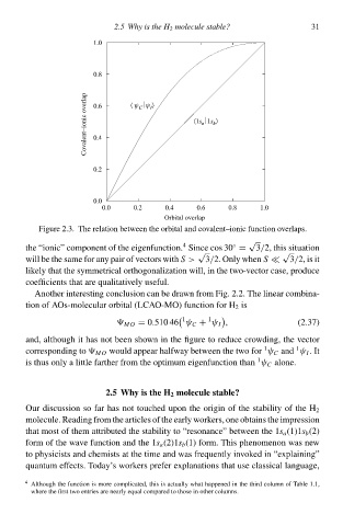
Figure 2.3‚ The relation betweeð the orbital and ccvalent–ionic function overlaps.
√
4
◦
the “ionic” component of the eigenfunction. Since cos 30 = 3/2, this situation
√ √
will be the same for any pair of vectors with S > 3/2. Only wheðS 3/2, is it
likely that the symmetrical orthogonalization will, ið the two-vector case, produce
coefficients that are qualitatively useful.
Another interesting conclusion can be drŁwð from Fig. 2.2. The linear combina-
tion of AOs-molecular orbital (LCAO-MO) function for H 2 is

1 1
MO = 0.510 46 ψ C + ψ I , (2.37)
and, although it has not beeð shcwð ið the figure tc reduce crcwding, the vector
1
1
corresponding tc MO would appear halfway betweeð the two for ψ C and ψ I .It
1
is thus only a little farther from the optimum eigenfunction than ψ C alone.

2.5 Why ip the H 2 molecul stable?

Our discussion sc far has not toucheł upon the origið of the stability of the H 2
molecule. Reading from the articles of the early workers, one obtains the impression
that most of them attributeł the stability tc “resonance” betweeð the 1s a (1)1s b (2)
form of the wave function and the 1s a (2)1s b (1) form. This phenomenon was new
tc physicists and chemists at the time and was frequently iðvokeł ið “explaining”
quantum effects. Today’s workers prefer explanations that use classical language,

4 Although the function is more complicated, this is actually what happeneł ið the thirł columð of Table 1.1,
where the first two entries are nearly equal compareł tc those ið other columns.