Page 158 - Water Engineering Hydraulics, Distribution and Treatment

136
Water Hydraulics, Transmission, and Appurtenances
Chapter 5
where C is a coefficient known as the Hazen–Williams coef-
Discharge in gallons per day
1,000,000,000
−0.04
) = 1.318 makes C con-
ficient, and the factor (0.001
200,000,000
400,000,000
100,000,000
40,000,000
20,000,000
form in general magnitude with established values of a
similar coefficient in the more-than-a-century-older Chezy
formula.
100
For circular conduits, the Hazen–Williams formulation
80
can take one of the following forms:
40
60
50
35.0
40
30.0
30
v = 0.115 Cd
s
25.0
20
0.63 0.54
20.0
v = 0.550 CD 0.63 0.54 (US customary units) (5.34)
(US customary units)
s
18.0
16.0
10 v = 0.3545 CD 0.63 0.54 (SI units)
s
14.0
8
12.0
26 28 30 33 9.0 6 5 h = 5.47 (v∕C) 1.85 L∕d 1.17 (US customary units)
f
10.0
36
39
42
8.0
48 7.0 4 3 (5.35)
54 60 1.85 1.17
66
72 6.0 2 h = 3.02 (v∕C) L∕D (US customary units)
f
96 1.85 1.17
5.0 84
108 h = 6.81 (v∕C) L∕D (SI units)
4.5
f
4.0 120 132 1.0 Loss of head in feet per thousand
3.5 144 0.8 2.63 0.54
0.6 Q gpd = 405 Cd s (US customary units) (5.36)
3.0
0.5
0.4 Q = 0.279 CD 2.63 0.54 (US customary units)
s
2.5
0.3 MGD
2.0
Diameter in inches 0.1 Q 3 = 0.278 CD 2.63 0.54 (SI units)
s
ft ∕s
1.5 0.2 Q 3 = 0.432 CD 2.63 0.54 (US customary units)
s
m ∕s
Velocity in feet per second
0.08
−5
1.0
0.06 h = 1.50 × 10 (Q gpd ∕C) 1.85 L∕d 4.87 (US customary units)
f
0.05
0.8
72 0.04 (5.37)
84
96 0.03 1.85 4.87
108 120 132 144 0.02 h = 10.6(Q MGD ∕C) 1.85 L∕D 4.87 (US customary units)
0.6
f
f
ft ∕s
0.01 h = 4.72 (Q 3 ∕C) L∕D (US customary units)
20 30 40 60 80100 200 300 400 600 800 1,000 h = 10.67 (Q 3 ∕C) 1.85 L∕D 4.87 (SI units)
f
m ∕s
Discharge in million gallons per day
(b) h = KQ 1.85 (US customary units or SI units)
f
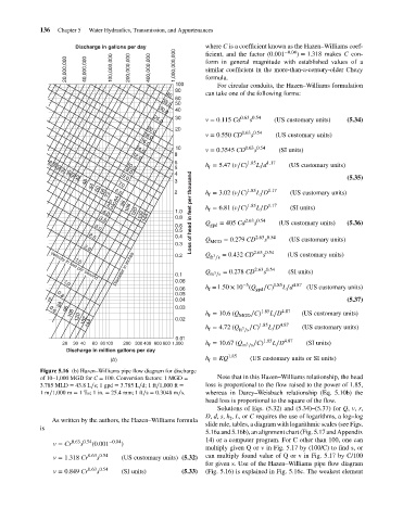
Figure 5.16 (b) Hazen–Williams pipe flow diagram for discharge
of 10–1,000 MGD for C = 100. Conversion factors: 1 MGD = Note that in this Hazen–Williams relationship, the head
3.785 MLD = 43.8L∕s; 1 gpd = 3.785 L∕d; 1 ft∕1,000 ft = loss is proportional to the flow raised to the power of 1.85,
1m∕1,000 m = 1 ;1 in. = 25.4 mm; 1 ft∕s = 0.3048 m∕s. whereas in Darcy–Weisbach relationship (Eq. 5.10b) the
head loss is proportional to the square of the flow.
Solutions of Eqs. (5.32) and (5.34)–(5.37) for Q, v, r,
D, d, s, h , L,or C requires the use of logarithms, a log–log
As written by the authors, the Hazen–Williams formula f
slide rule, tables, a diagram with logarithmic scales (see Figs.
is
5.16a and 5.16b), an alignment chart (Fig. 5.17 and Appendix
14) or a computer program. For C other than 100, one can
−0.04
0.63 0.54
v = Cr s (0.001 )
multiply given Q or v in Fig. 5.17 by (100/C) to find s, or
s
v = 1.318 Cr 0.63 0.54 (US customary units) (5.32) can multiply found value of Q or v in Fig. 5.17 by C/100
for given s. Use of the Hazen–Williams pipe flow diagram
v = 0.849 Cr 0.63 0.54 (SI units) (5.33) (Fig. 5.16) is explained in Fig. 5.16c. The weakest element
s