Page 159 - Water Engineering Hydraulics, Distribution and Treatment

Q
v = 3 ft/s
d = 12"
d = 24"
2.07
s
0.12
(ii)
(i)
1.0
Q
Q
d = 14" d = 12"
(2)
25.3
(3)
(3)
2.8
d = 10"
2.1
s
d = 8"
(1)
d = 10"
(1)
(iv) 2.9 s s d = 16" (2) 1.33 Q (3) d = 18" (1) (v) 5.4 s s v = 2 ft/s d = 36" Q Q (3) (1) (iii) (vi) 0.9 54.0
1.012 2.980 4.250 2.03.0
(c)
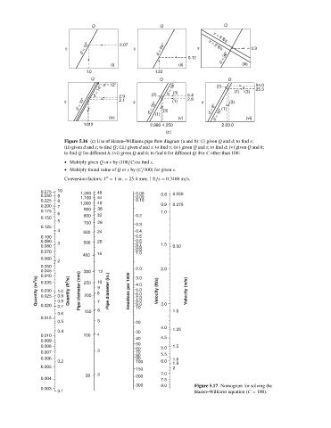
Figure 5.16 (c) Use of Hazen–Williams pipe flow diagram (a and b): (i) given Q and d;tofind s;
(ii) given d and s;tofind Q; (iii) given d and s;tofind v; (iv) given Q and s;tofind d; (v) given Q and h;
to find Q for different h;(vi)given Q and h;tofind h for different Q.For C other than 100:
Multiply given Q or v by (100∕C)tofind s.

Multiply found value of Q or v by (C∕100) for given s.

′′
Conversion factors: 1 = 1in. = 25.4 mm; 1 ft∕s = 0.3408 m∕s.
0.275 10 1,200 48 0.08
0.250 9 1,100 44 0.09 0.8 0.250
0.225 8 0.10
1,000 40
0.200 7 36 0.9 0.275
0.175 900 1.0
6 32
0.150 800 0.2
5
700 28 0.3
0.125
4 600 24 0.4
0.100 0.5
0.090 3 500 20 0.6
0.080 0.7 1.5 0.50
0.8
0.070 16 0.9
1.0
400
0.060
2
0.050 2.0
0.045 300 12 2.0
0.040 250 10 3.0
Quantity (m 3 /s) 0.030 1.0 Quantity (ft 3 /s) Pipe diameter (mm) 200 9 8 7 Pipe diameter (in.) Headloss per 1000 4.0 Velocity (ft/s) Velocity (m/s)
0.035
5.0
6.0
0.9
0.025
7.0
8.0
0.8
0.020
0.7
10
0.6 150 6 9.0 3.0 1.0
0.015
0.5 5 20
4.0 1.25
0.4 30
0.010 100 4
40 4.5
0.009
50
0.008 60 5.0 1.5
0.007 3 70
80 5.5
0.006 90 1.8
0.2 100 6.0 1.9
0.005
150 2
50 2 200 7.0
0.004 7.5
300 8.0 Figure 5.17 Nomogram for solving the
0.003
0.1 Hazen–Williams equation (C = 100).