Page 85 - Water Engineering Hydraulics, Distribution and Treatment

63
3.12 Multiple-Well Systems
3
Q
3
transmissivity in m /d/m.
Q
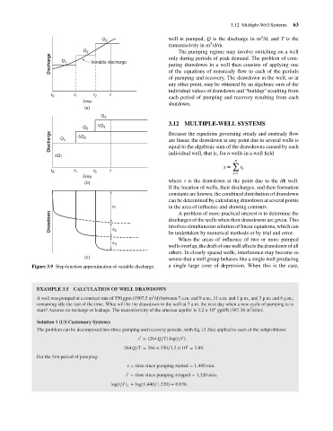
The pumping regime may involve switching on a well
2
Discharge
only during periods of peak demand. The problem of com-
Q
Variable discharge
1
puting drawdown in a well then consists of applying one
of the equations of nonsteady flow to each of the periods
of pumping and recovery. The drawdown in the well, or at
any other point, may be obtained by an algebraic sum of the
individual values of drawdown and “buildup” resulting from
t
t
t
2
0
1
each period of pumping and recovery resulting from each
Time
shutdown.
(a)
Q 3 3 t well is pumped, Q is the discharge in m /d, and T is the
Q 2 ΔQ 3 3.12 MULTIPLE-WELL SYSTEMS
Discharge Q 1 ΔQ 2 are linear, the drawdown at any point due to several wells is
Because the equations governing steady and unsteady flow
equal to the algebraic sum of the drawdowns caused by each
ΔQ 1 individual well, that is, for n wells in a well field
n
∑
s = s i
t 0 t 1 t 2 t i=1
Time
where s is the drawdown at the point due to the ith well.
(b)
If the location of wells, their discharges, and their formation
constants are known, the combined distribution of drawdown
can be determined by calculating drawdown at several points
s 1 in the area of influence and drawing contours.
Drawdown discharges of the wells when their drawdowns are given. This
A problem of more practical interest is to determine the
involves simultaneous solution of linear equations, which can
s
2
be undertaken by numerical methods or by trial and error.
When the areas of influence of two or more pumped
s 3
wells overlap, the draft of one well affects the drawdown of all
others. In closely spaced wells, interference may become so
(c)
severe that a well group behaves like a single well producing
Figure 3.9 Step function approximation of variable discharge. a single large cone of depression. When this is the case,
EXAMPLE 3.5 CALCULATION OF WELL DRAWDOWN
3
A well was pumped at a constant rate of 350 gpm (1907.5 m /d) between 7 a.m. and 9 a.m., 11 a.m. and 1 p.m., and 3 p.m. and 6 p.m.,
remaining idle the rest of the time. What will be the drawdown in the well at 7 a.m. the next day when a new cycle of pumping is to
3
4
start? Assume no recharge or leakage. The transmissivity of the artesian aquifer is 3.2 × 10 gpd/ft (397.38 m /d/m).
Solution 1 (US Customary System):
The problem can be decomposed into three pumping and recovery periods, with Eq. (3.26a) applied to each of the subproblems:
′ ′
s = (264 Q∕T) log(t∕t ).
4
264 Q∕T = 264 × 350∕3.2 × 10 = 2.89.
For the first period of pumping:
t = time since pumping started = 1,440 min.
′
t = time since pumping stopped = 1,320 min.
′
log(t∕t ) =log(1,440∕1,320) = 0.038.
1