Page 82 - Water Engineering Hydraulics, Distribution and Treatment

60
Chapter 3
Water Sources: Groundwater
2
10
Nonequilibrium
type curve
10
0.01
0.03
0.075
0.1
W (u, r/B)
10
T
2
1.87 r S
u =
Tt
2.0 1.5 1.0 0.8 0.7 0.6 0.5 0.4 0.3 0.2 s = 0.15 114.6 Q W(u, r/B) 0.05 0.015 0.005 0.001
r r
r/B = 2.5 =
0.1 B T
(k´/b´ )
0.01
10 –1 1.0 10 10 2 10 3 10 4 10 5 10 6 10 7
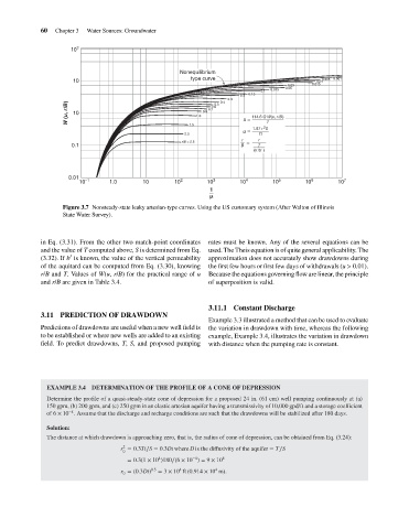
Figure 3.7 Nonsteady-state leaky artesian-type curves. Using the US customary system (After Walton of Illinois
State Water Survey).
in Eq. (3.31). From the other two match-point coordinates rates must be known. Any of the several equations can be
and the value of T computed above, S is determined from Eq. used. The Theis equation is of quite general applicability. The
′
(3.32). If b is known, the value of the vertical permeability approximation does not accurately show drawdowns during
of the aquitard can be computed from Eq. (3.30), knowing the first few hours or first few days of withdrawals (u > 0.01).
r/B and T. Values of W(u, r/B) for the practical range of u Because the equations governing flow are linear, the principle
and r/B are given in Table 3.4. of superposition is valid.
3.11.1 Constant Discharge
3.11 PREDICTION OF DRAWDOWN
Example 3.3 illustrated a method that can be used to evaluate
Predictions of drawdowns are useful when a new well field is the variation in drawdown with time, whereas the following
to be established or where new wells are added to an existing example, Example 3.4, illustrates the variation in drawdown
field. To predict drawdowns, T, S, and proposed pumping with distance when the pumping rate is constant.

EXAMPLE 3.4 DETERMINATION OF THE PROFILE OF A CONE OF DEPRESSION
Determine the profile of a quasi-steady-state cone of depression for a proposed 24 in. (61 cm) well pumping continuously at (a)
150 gpm, (b) 200 gpm, and (c) 250 gpm in an elastic artesian aquifer having a transmissivity of 10,000 gpd/ft and a storage coefficient
−4
of 6 × 10 . Assume that the discharge and recharge conditions are such that the drawdowns will be stabilized after 180 days.
Solution:
The distance at which drawdown is approaching zero, that is, the radius of cone of depression, can be obtained from Eq. (3.24):
2
r = 0.3Tt∕S = 0.3Dt where D is the diffusivity of the aquifer = T∕S
0
4
−4
= 0.3(1 × 10 )180∕(6 × 10 ) = 9 × 10 8
4
4
r = (0.3Dt) 0.5 = 3 × 10 ft (0.914 × 10 m).
0