Page 77 - Water Engineering Hydraulics, Distribution and Treatment

Compute the formation constants:
T = 114.6 × 350 × 4.0∕5.0
4
T = 3.2 × 10 gpd∕ft
2
S = uT∕(1.87 r ∕t)
−2
S = 10
(3.2 × 10 )∕[1.87(5 × 10 )]
−5
S = 3.4 × 10 .
Solution 2 (SI System): T = 114.6QW(u)∕s 4 6 3.10 Nonsteady Radial Flow 55
T = [Q∕(4 s)]W(u)
T = [1808∕4 × 3.14 × 1.524)] × 4
3
T = 398.72 m ∕d∕m
2
S = 4 Tu∕(r ∕t)
5
−2
S = 4 × 398.72 × 10 ∕(4.645 × 10 )
−5
S = 3.43 × 10 .
EXAMPLE 3.2 CALCULATIONS OF DRAWDOWN WITH TIME IN A WELL
In the aquifer represented by the pumping test in Example 3.1, a gravel-packed well with an effective diameter of 24 in. (610 mm) is
3
to be constructed. The design flow of the well is 700 gpm (3,815 m /d). Calculate the drawdown at the well with total withdrawals
from storage (i.e., with no recharge or leakages) after (a) 1 minute, (b) 1 hour, (c) 8 hours, (d) 24 hours, (e) 30 days, and (f) 6 months
of continuous pumping, at design capacity.
Solution 1 (US Customary System):
From Eq. (3.15): s = [114.6 Q∕T][W(u)]
4
= [114.6 × 700∕(3.2 × 10 )][W(u)]
= 2.51 ft [W(u)].
2
From Eq. (3.16): u = 1.87 r S∕Tt
−5
2
4
= 1.87 × 1 × 3.4 × 10 ∕(3.2 × 10 )t
−9
= (2.0 × 10 )∕t.
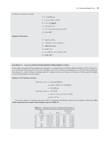
For various values of t, compute u, then from Table 3.2 obtain the well function, W(u), for the calculation of drawdown. The
values of drawdown for various values of time are given in Table 3.3.

Table 3.3 Variation of drawdown with time for Example 3.2
Time Drawdown,
(days) u W(u) s,ft(m)
(a) 1/1,440 2.86 × 10 −6 12.19 30.6 (9.33)
(b) 1/24 4.8 × 10 −8 16.27 40.8 (12.44)
(c) 1/3 6.0 × 10 −9 18.35 46.0 (14.02)
(d) 1 2.0 × 10 −9 19.45 48.8 (14.87)
(e) 30 6.6 × 10 −11 22.86 57.3 (17.46)
(f) 180 1.1 × 10 −11 24.66 61.8 (18.84)