Page 75 - Water Engineering Hydraulics, Distribution and Treatment

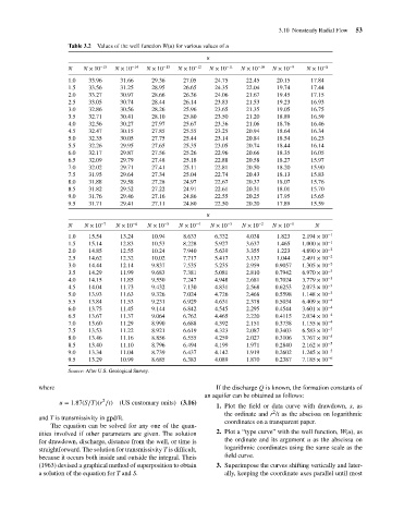
3.10 Nonsteady Radial Flow
Table 3.2
u
−13
−14
−12
−15
N × 10
N × 10
N
N × 10
N × 10
27.05
29.36
20.15
22.45
33.96
24.75
1.0
17.84
31.66
19.74
24.35
28.95
17.44
31.25
1.5
33.56
22.04
26.65
24.06
26.36
30.97
28.66
33.27
2.0
21.67
19.45
17.15
30.74
19.23
33.05
2.5
26.14
28.44
23.83
16.93
21.53
28.26
16.75
32.86
30.56
3.0
19.05
25.96
23.65
21.35
30.41
21.20
28.10
16.59
23.50
25.80
3.5
32.71
18.89
18.76
16.46
32.56
23.36
27.97
25.67
21.06
30.27
4.0
20.94
18.64
25.55
16.34
23.25
27.85
30.15
32.47
4.5
25.44
20.84
16.23
23.14
5.0 N × 10 Values of the well function W(u) for various values of u −11 N × 10 −10 N × 10 −9 N × 10 −8 53
18.54
30.05
27.75
32.35
5.5 32.26 29.95 27.65 25.35 23.05 20.74 18.44 16.14
6.0 32.17 29.87 27.56 25.26 22.96 20.66 18.35 16.05
6.5 32.09 29.79 27.48 25.18 22.88 20.58 18.27 15.97
7.0 32.02 29.71 27.41 25.11 22.81 20.50 18.20 15.90
7.5 31.95 29.64 27.34 25.04 22.74 20.43 18.13 15.83
8.0 31.88 29.58 27.28 24.97 22.67 20.37 18.07 15.76
8.5 31.82 29.52 27.22 24.91 22.61 20.31 18.01 15.70
9.0 31.76 29.46 27.16 24.86 22.55 20.25 17.95 15.65
9.5 31.71 29.41 27.11 24.80 22.50 20.20 17.89 15.59
u
N N × 10 −7 N × 10 −6 N × 10 −5 N × 10 −4 N × 10 −3 N × 10 −2 N × 10 −1 N
1.0 15.54 13.24 10.94 8.633 6.332 4.038 1.823 2.194 × 10 −1
1.5 15.14 12.83 10.53 8.228 5.927 3.637 1.465 1.000 × 10 −1
2.0 14.85 12.55 10.24 7.940 5.639 3.355 1.223 4.890 × 10 −2
2.5 14.62 12.32 10.02 7.717 5.417 3.137 1.044 2.491 × 10 −2
3.0 14.44 12.14 9.837 7.535 5.235 2.959 0.9057 1.305 × 10 −2
3.5 14.29 11.99 9.683 7.381 5.081 2.810 0.7942 6.970 × 10 −3
4.0 14.15 11.85 9.550 7.247 4.948 2.681 0.7024 3.779 × 10 −3
4.5 14.04 11.73 9.432 7.130 4.831 2.568 0.6253 2.073 × 10 −3
5.0 13.93 11.63 9.326 7.024 4.726 2.468 0.5598 1.148 × 10 −3
5.5 13.84 11.53 9.231 6.929 4.631 2.378 0.5034 6.409 × 10 −4
6.0 13.75 11.45 9.144 6.842 4.545 2.295 0.4544 3.601 × 10 −4
6.5 13.67 11.37 9.064 6.762 4.465 2.220 0.4115 2.034 × 10 −4
7.0 13.60 11.29 8.990 6.688 4.392 2.151 0.3738 1.155 × 10 −4
7.5 13.53 11.22 8.921 6.619 4.323 2.087 0.3403 6.583 × 10 −5
8.0 13.46 11.16 8.856 6.555 4.259 2.027 0.3106 3.767 × 10 −5
8.5 13.40 11.10 8.796 6.494 4.199 1.971 0.2840 2.162 × 10 −5
9.0 13.34 11.04 8.739 6.437 4.142 1.919 0.2602 1.245 × 10 −5
9.5 13.29 10.99 8.685 6.383 4.089 1.870 0.2387 7.185 × 10 −6
Source: After U.S. Geological Survey.
where If the discharge Q is known, the formation constants of
an aquifer can be obtained as follows:
2
u = 1.87(S∕T)(r ∕t) (US customary units) (3.16)
1. Plot the field or data curve with drawdown, s,as
2
the ordinate and r /t as the abscissa on logarithmic
and T is transmissivity in gpd/ft.
coordinates on a transparent paper.
The equation can be solved for any one of the quan-
tities involved if other parameters are given. The solution 2. Plot a “type curve” with the well function, W(u), as
for drawdown, discharge, distance from the well, or time is the ordinate and its argument u as the abscissa on
straightforward. The solution for transmissivity T is difficult, logarithmic coordinates using the same scale as the
because it occurs both inside and outside the integral. Theis field curve.
(1963) devised a graphical method of superposition to obtain 3. Superimpose the curves shifting vertically and later-
a solution of the equation for T and S. ally, keeping the coordinate axes parallel until most