Page 79 - Water Engineering Hydraulics, Distribution and Treatment

EXAMPLE 3.3 DETERMINATION OF THE T AND S COEFFICIENTS OF AN AQUIFER USING THE
APPROXIMATION METHOD
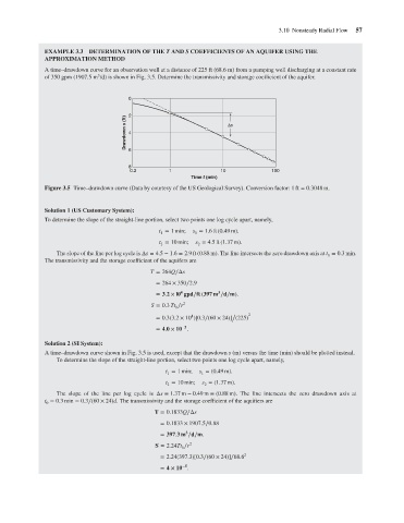
A time–drawdown curve for an observation well at a distance of 225 ft (68.6 m) from a pumping well discharging at a constant rate
3
of 350 gpm (1907.5 m /d) is shown in Fig. 3.5. Determine the transmissivity and storage coefficient of the aquifer.
Drawdown s (ft) 0 2 4 6 Δs 3.10 Nonsteady Radial Flow 57
8
0.2 1 10 100
Time t (min)
Figure 3.5 Time–drawdown curve (Data by courtesy of the US Geological Survey). Conversion factor: 1 ft = 0.3048 m.

Solution 1 (US Customary System):
To determine the slope of the straight-line portion, select two points one log cycle apart, namely,
t = 1 min; s = 1.6ft(0.49 m).
1
1
t = 10 min; s = 4.5ft(1.37 m).
2
2
The slope of the line per log cycle is Δs = 4.5 − 1.6 = 2.9ft(0.88 m). The line intersects the zero drawdown axis at t = 0.3 min.
0
The transmissivity and the storage coefficient of the aquifers are
T = 264Q∕Δs
= 264 × 350∕2.9
4 3
= 3.2 × l0 gpd∕ft (397 m ∕d∕m).
S = 0.3 Tt ∕r 2
0
/
4
= 0.3(3.2 × 10 )[0.3∕(60 × 24)] (225) 2
−5
= 4.0 × 10 .
Solution 2 (SI System):
A time–drawdown curve shown in Fig. 3.5 is used, except that the drawdown s (m) versus the time (min) should be plotted instead.
To determine the slope of the straight-line portion, select two points one log cycle apart, namely,
t = 1 min; s = (0.49 m).
1
1
t = 10 min; s = (1.37 m).
2
2
The slope of the line per log cycle is Δs = 1.37 m − 0.49 m = (0.88 m). The line intersects the zero drawdown axis at
t = 0.3 min = 0.3∕(60 × 24)d. The transmissivity and the storage coefficient of the aquifiers are
0
T = 0.1833Q∕Δs
= 0.1833 × 1907.5∕0.88
3
= 397.3m ∕d∕m.
S = 2.24Tt ∕r 2
0
= 2.24(397.3)[0.3∕(60 × 24)]∕68.6 2
−5
= 4 × 10 .