Page 49 - Fluid Power Engineering

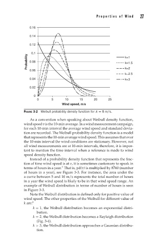
Properties of W ind 27

0.16

0.14
0.12

0.1 k=1
Probability 0.08 k=1.5

0.06 k=2
k=2.5
0.04 k=3

0.02

0
0 5 10 15 20 25
Wind speed, m/s
FIGURE 3-2 Weibull probability density function for A = 8 m/s.
As a convention when speaking about Weibull density function,
windspeedvisthe10-minaverage.Inawindmeasurementcampaign,
for each 10-min interval the average wind speed and standard devia-
tion are recorded. The Weibull probability density function is a model
that represents the 10-min average wind speed. This assumes that over
the 10-min interval the wind conditions are stationary. However, not
all wind measurements are at 10-min intervals, therefore, it is impor-
tant to mention the time interval when a reference is made to wind
speed density function.
Instead of a probability density function that represents the frac-
tion of time wind speed is at v, it is sometimes customary to speak in
1
terms of hours in a year. That is, pd(v) is multiplied by 8760 (number
of hours in a year), see Figure 3-3. For instance, the area under the
a curve between 5 and 10 m/s represents the total number of hours
in a year the wind speed is likely to be in that wind speed range. An
example of Weibull distribution in terms of number of hours is seen
in Figure 3-3.
Note the Weibull distribution is defined only for positive value of
wind speed. The other properties of the Weibull for different value of
k are: 1
k = 1, the Weibull distribution becomes an exponential distri-
bution.
k = 2, the Weibull distribution becomes a Rayleigh distribution
(Fig. 3-4).
k > 3, the Weibull distribution approaches a Gaussian distribu-
tion.