Page 277 - Wind Energy Handbook

BLADE LOADS DURING OPERATION 251

As with the elements of the S matrix, the elements of the H matrix are all double-
sided functions of frequency, n.
Noting that the expression for the power spectral density S kk resembles that for
the variance of the sum of group of k independent variables, it is apparent that the
elements of the H matrix can be considered as the weighting factors for the linear
combination of N independent, unit magnitude, white noise inputs to yield N
correlated outputs with the correct spectral matrix. Thus the elements in the jth
row of H are the weighting factors for the inputs contributing to the output at point
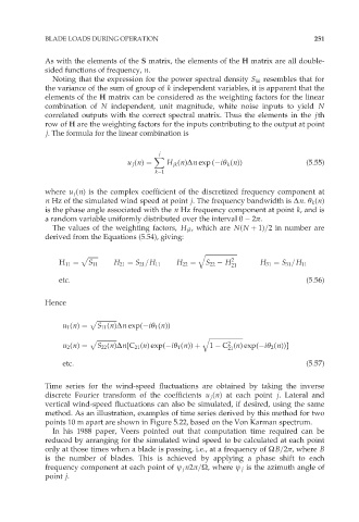
j. The formula for the linear combination is

j
X
u j (n) ¼ H jk (n)˜n exp ( iŁ k (n)) (5:55)
k¼1

where u j (n) is the complex coefficient of the discretized frequency component at
n Hz of the simulated wind speed at point j. The frequency bandwidth is ˜n. Ł k (n)
is the phase angle associated with the n Hz frequency component at point k, and is
a random variable uniformly distributed over the interval 0 2ð.
The values of the weighting factors, H jk , which are N(N þ 1)=2 in number are
derived from the Equations (5.54), giving:

p ffiffiffiffiffiffiffi q ffiffiffiffiffiffiffiffiffiffiffiffiffiffiffiffiffiffiffiffiffi
H 11 ¼ S 11 H 21 ¼ S 21 =H 11 H 22 ¼ S 22 H 2 H 31 ¼ S 31 =H 11
21
etc: (5:56)

Hence
p ffiffiffiffiffiffiffiffiffiffiffiffiffi
u 1 (n) ¼ S 11 (n)˜n exp( iŁ 1 (n))

p ffiffiffiffiffiffiffiffiffiffiffiffiffi q ffiffiffiffiffiffiffiffiffiffiffiffiffiffiffiffiffiffiffiffiffiffi
2
u 2 (n) ¼ S 22 (n)˜n[C 21 (n) exp( iŁ 1 (n)) þ 1 C (n) exp( iŁ 2 (n))]
21
etc: (5:57)

Time series for the wind-speed fluctuations are obtained by taking the inverse
discrete Fourier transform of the coefficients u j (n) at each point j. Lateral and
vertical wind-speed fluctuations can also be simulated, if desired, using the same
method. As an illustration, examples of time series derived by this method for two
points 10 m apart are shown in Figure 5.22, based on the Von Karman spectrum.
In his 1988 paper, Veers pointed out that computation time required can be
reduced by arranging for the simulated wind speed to be calculated at each point
only at those times when a blade is passing, i.e., at a frequency of ÙB=2ð, where B
is the number of blades. This is achieved by applying a phase shift to each
frequency component at each point of ł j n2ð=Ù, where ł j is the azimuth angle of
point j.