Page 369 - Characterization and Properties of Petroleum Fractions - M.R. Riazi

P1: JDW
June 22, 2007
AT029-Manual
14:25
AT029-Manual-v7.cls
AT029-08
8. APPLICATIONS: ESTIMATION OF TRANSPORT PROPERTIES 349
reduced diffusivity and reduced viscosity [9]:
1.2
b+cP r
_- (ρD AB) μ

1.0 (ρD AB) ◦ = a b =−0.27 − 0.38ω
μ
◦
Reduced Density -Diffusivity, (ρD/ρD) o 0.8 (8.67) T c = x A T cA + x B T cB P r = P/P c ◦
a = 1.07
c =−0.05 + 0.1ω
P c = x A P cA + x B P cB
0.6
ω = x A ω A + x B ω B
where (ρD AB) must be determined from Eq. (8.57). μ must
0.4
◦
on μ are not available it should be calculated from Eq. (8.12)
0.2 be calculated from Eqs. (8.6) and (8.8). If experimental data
for both liquids and gases. Coefficients a, b, and c have
been determined from data on diffusion coefficients of some
0.0 300 binary systems as shown in Table 8.10. Errors for both
0.1 1 10 Eqs. (8.65) and (8.67) are also shown in this table. In eval-
Reduced Density, ρ/ρ uation of Eq. (8.65) the coefficients were reevaluated from
C
the same data bank as given in Table 8.10. When Eq. (8.67) is
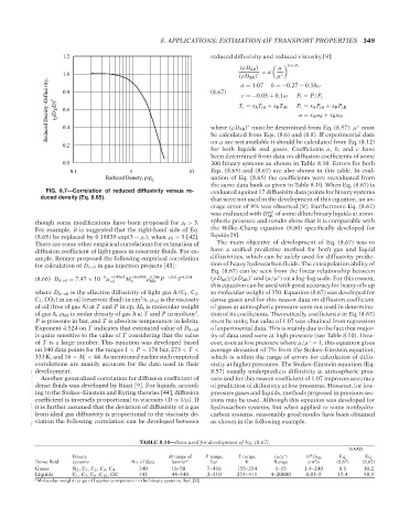
FIG. 8.7—Correlation of reduced diffusivity versus re- evaluated against 17 diffusivity data points for binary systems
duced density (Eq. 8.65). that were not used in the development of this equation, an av-
erage error of 9% was observed [9]. Furthermore Eq. (8.67)
was evaluated with D AB of some dilute binary liquids at atmo-
∞L
though some modifications have been proposed for ρ r > 3. spheric pressure and results show that it is comparable with
For example, it is suggested that the right-hand side of Eq. the Wilke–Chang equation (8.60) specifically developed for
(8.65) be replaced by 0.18839 exp(3 − ρ r ), when ρ r > 3 [42]. liquids [9].
There are some other empirical correlations for estimation of The main objective of development of Eq. (8.67) was to
diffusion coefficient of light gases in reservoir fluids. For ex- have a unified predictive method for both gas and liquid
ample, Renner proposed the following empirical correlation diffusivities, which can be safely used for diffusivity predic-
for calculation of D i-oil in gas injection projects [43]: tion of heavy hydrocarbon fluids. The extrapolation ability of
Eq. (8.67) can be seen from the linear relationship between
−8
◦
(8.66) D A-oil = 7.47 × 10 μ −0.4562 M −0.6898 1.706 P −1.831 T 4.524 (ρD AB)/(ρD AB) and (μ/μ ) on a log–log scale. For this reason,
◦
ρ
oil A MA
this equation can be used with good accuracy for heavy oils up
where D A−oil is the effective diffusivity of light gas A (C 1 ,C 2 , to molecular weight of 350. Equation (8.67) was developed for
2
C 3 ,CO 2 ) in an oil (reservoir fluid) in cm /s. μ oil is the viscosity dense gases and for this reason data on diffusion coefficient
of oil (free of gas A) at T and P in cp, M A is molecular weight of gases at atmospheric pressure were not used in determina-
3
of gas A, ρ MA is molar density of gas A at T and P in mol/cm , tion of its coefficients. Theoretically, coefficient a in Eq. (8.67)
P is pressure in bar, and T is absolute temperature in kelvin. must be unity, but value of 1.07 was obtained from regression
Exponent 4.524 on T indicates that estimated value of D A−oil of experimental data. This is mainly due to the fact that major-
is quite sensitive to the value of T considering that the value ity of data used were at high pressure (see Table 8.10). How-
of T is a large number. This equation was developed based ever, even at low pressure where μ/μ = 1, this equation gives
◦
on 140 data points for the ranges 1 < P < 176 bar, 273 < T < average deviation of 7% from the Stokes–Einstein equation,
333 K, and 16 < M i < 44. As mentioned earlier such empirical which is within the range of errors for calculation of diffu-
correlations are mainly accurate for the data used in their sivity at higher pressures. The Stokes–Einstein equation (Eq.
development. 8.57) usually underpredicts diffusivity at atmospheric pres-
Another generalized correlation for diffusion coefficient of sure and for this reason coefficient of 1.07 improves accuracy
dense fluids was developed by Riazi [9]. For liquids, accord- of prediction of diffusivity at low pressures. However, for low-
ing to the Stokes–Einstein and Eyring theories [44], diffusion pressure gases and liquids, methods proposed in previous sec-
coefficient is inversely proportional to viscosity (D ∝ 1/μ). If tions may be used. Although this equation was developed for
it is further assumed that the deviation of diffusivity of a gas hydrocarbon systems, but when applied to some nonhydro-
from ideal gas diffusivity is proportional to the viscosity de- carbon systems, reasonably good results have been obtained
viation the following correlation can be developed between as shown in the following example.
--`,```,`,``````,`,````,```,,-`-`,,`,,`,`,,`---
TABLE 8.10—Data used for development of Eq. (8.67).
%AAD
4
Binary M range of P range, T range, (μ/μ ) 10 D AB , Eq. Eq.
◦
2
Dense fluid systems No. of data barrier a bar K Range cm /s (8.67) (8.65)
Gases N 2 ,C 1 ,C 2 ,C 3 ,C 4 140 16–58 7–416 155–354 1–15 1.4–240 8.1 10.2
Liquids C 1 ,C 3 ,C 6 ,C 10 , Oil 143 44–340 2–310 274–411 4–20000 0.01–5 15.4 48.9
a Molecular weight range of heavier component in the binary systems. Ref. [9].

Copyright ASTM International
Provided by IHS Markit under license with ASTM Licensee=International Dealers Demo/2222333001, User=Anggiansah, Erick
No reproduction or networking permitted without license from IHS Not for Resale, 08/26/2021 21:56:35 MDT