Page 370 - Characterization and Properties of Petroleum Fractions - M.R. Riazi

P1: JDW
June 22, 2007
14:25
AT029-Manual
AT029-08
AT029-Manual-v7.cls
350 CHARACTERIZATION AND PROPERTIES OF PETROLEUM FRACTIONS
Example 8.4—Estimate the diffusivity of benzene in a binary
mixture of 74.2 mol% acetone and 25.8 mol% carbon tetra- For a ternary system of C 1 –C 3 –N 2 at low pressure, the effec-
tive diffusion coefficient of C 1 in the mixture calculated from
chloride (CCl 4 ) at 298 K and 1 atm pressure. Eq. (8.69) differs by 2–3% from Eq. (8.68) for mole fraction
range of 0.0–0.5 [9]. Application of Eq. (8.69) was previously
Solution—The system is a ternary mixture of benzene, shown in Example 8.4.
acetone, and CCl 4 . Consider benzene, the solute, as compo-
nent A and the mixture of acetone and CCl 4 , the solvent, as
component B. Because amount of benzene is small (dilute 8.3.5 Diffusion Coefficient in Porous Media
system), x A = 0.0 and x B = 1.0. T cB = 520, P cB = 46.6 bar, The predictive methods presented in this section are appli-
3
V cB = 226.3cm /mol, ω = 0.2274, M = 82.8. These prop- cable to normal media fully filled by the fluid of interest. In
erties are calculated from properties of acetone and CCl 4 catalytic reactions and hydrocarbon reservoirs, the fluid is
as given in Ref. [45]. Actually the liquid solvent is the within a porous media and as a result for molecules it takes
same as the liquid in Example 8.1, calculated properties longer time to travel a specific length in order to diffuse. This
3
◦
of which are ρ = 0.012422 mol/cm , μ = 0.00829 and μ = in turn would result in lowering diffusion coefficient. The
◦
0.374, thus μ/μ = 45.1677. From Eq. (8.67), b =−0.356, c = effective diffusion coefficient in a porous media, D AB,eff can
◦
−0.02726, and (ρD AB)/(ρD AB) = 0.2745. From Eq. (8.57), be calculated as
◦
(ρD AB) = 1.28 × 10 −6 mol/cm · s. Therefore, D AB = 1.28 ×
2
10 −6 × 0.2745/0.012422 = 2.83 × 10 −5 cm /s. In comparison (8.70) D AB,eff = D AB
2
with the experimental value of 2.84 × 10 −5 cm /s [10] an error τ n
of −0.4% is obtained. In this example both μ and ρ have been where D AB is the diffusion coefficient in absence of porous me-
calculated, while in many cases these values may be known dia and exponent n is usually taken as one but other values of
from experimental measurements. nare also recommended for some porous media systems [47].
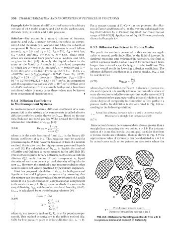
τ is a dimensionless parameter called tortuosity defined to in-
8.3.4 Diffusion Coefficients dicate degree of complexity in connection of free paths in a
in Mutlicomponent Systems porous media. Its definition is demonstrated in Fig. 8.8 ac-
cording to the following relation:
In multicomponent systems, diffusion coefficient of a com-
ponent (A) in the mixture of N components is called effective Actual free distance between points a and b in porous media
diffusion coefficient and is shown by D A-mix . Based on the ma- τ = Distance of a straight line between a and b
terial balance and ideal gas law Wilke derived the following (8.71)
relation for calculation of D A-mix [46]:
Since actual distance between a and b is always greater than a
(8.68) 1 − y A straight line connecting the two points, τ> 1.0. For determi-
N y i
D A-mix =
i =A D A-i nation of τ in an ideal media, assuming all particles that form
where y i is the mole fraction of i and D A−i is the binary dif- a porous media are spherical, then as shown in Fig. 8.9 the
∼
fusion coefficient of A in i. This equation may be used for approximate value of tortuosity can be calculated as τ = 1.4.
pressures up to 35 bar; however, because of lack of a reliable In actual cases such as for petroleum reservoirs where the
method, this is also used for high-pressure gases and liquids
as well [9]. For calculation of D A-mix in liquids the method
of Leffler and Cullinan is recommended in the API-TDB [5].
This method requires binary diffusion coefficients at infinite
∞L
dilution D A-i , mole fraction of each component x i , liquid
viscosity of each component μ i , and viscosity of liquid mix-
ture μ m . However, this method is not recommended in other
sources and is not widely practiced by petroleum engineers.
Riazi has proposed calculation of D A-mix for both gases and
liquids at low and high-pressure systems by assuming that
the mixture can be considered as a binary solution of A and B
where B is a pseudocomponent composed of all components
in the mixture except A. D A-mix is assumed to be the same as bi-
nary diffusivity, D AB , which can be calculated from Eq. (8.67).
D A-mix is calculated from the following relations [9]:
D A-mix = D AB
(8.69) N
i=1 x i θ i
i =A
θ B = N
i=1 x i Free distance between a and b
i =A τ=
Distance of straight line between a and b
where θ B is a property such as T c , P c ,or ω for pseudocompo-
nent B. This method is equivalent to the Wilke’s method (Eq. FIG. 8.8—Distance for traveling a molecule from a to b
8.68) for low-pressure gases at infinite dilution (i.e., x A → 0). in a porous media and concept of tortuosity.
--`,```,`,``````,`,````,```,,-`-`,,`,,`,`,,`---

Copyright ASTM International
Provided by IHS Markit under license with ASTM Licensee=International Dealers Demo/2222333001, User=Anggiansah, Erick
No reproduction or networking permitted without license from IHS Not for Resale, 08/26/2021 21:56:35 MDT