Page 423 - Mechanical Behavior of Materials

424 Chapter 9 Fatigue of Materials: Introduction and Stress-Based Approach

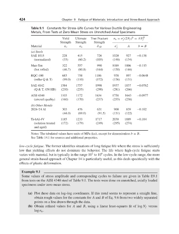
Table 9.1 Constants for Stress–Life Curves for Various Ductile Engineering
Metals, From Tests at Zero Mean Stress on Unnotched Axial Specimens
b

Yield Ultimate True Fracture σ a = σ (2N f ) = AN B
f f
Strength Strength Strength
Material σ A b = B
σ u
˜ σ fB
σ o
f
(a) Steels
SAE 1015 228 415 726 1020 927 −0.138
(normalized) (33) (60.2) (105) (148) (134)
Man-Ten 322 557 990 1089 1006 −0.115
(hot rolled) (46.7) (80.8) (144) (158) (146)
RQC-100 683 758 1186 938 897 −0.0648
(roller Q & T) (99.0) (110) (172) (136) (131)
SAE 4142 1584 1757 1998 1937 1837 −0.0762
(Q & T, 450 HB) (230) (255) (290) (281) (266)
AISI 4340 1103 1172 1634 1758 1643 −0.0977
(aircraft quality) (160) (170) (237) (255) (238)
(b) Other Metals
2024-T4 Al 303 476 631 900 839 −0.102
(44.0) (69.0) (91.5) (131) (122)
Ti-6Al-4V 1185 1233 1717 2030 1889 −0.104
(solution treated (172) (179) (249) (295) (274)
and aged)
Notes: The tabulated values have units of MPa (ksi), except for dimensionless b = B.
See Table 14.1 for sources and additional properties.

low-cycle fatigue. The former identifies situations of long fatigue life where the stress is sufficiently
low that yielding effects do not dominate the behavior. The life where high-cycle fatigue starts
4
2
varies with material, but is typically in the range 10 to 10 cycles. In the low-cycle range, the more
general strain-based approach of Chapter 14 is particularly useful, as this deals specifically with the
effects of plastic deformation.
Example 9.1
Some values of stress amplitude and corresponding cycles to failure are given in Table E9.1
from tests on the AISI 4340 steel of Table 9.1. The tests were done on unnotched, axially loaded
specimens under zero mean stress.

(a) Plot these data on log–log coordinates. If this trend seems to represent a straight line,
obtain rough values for the constants for A and B of Eq. 9.6 from two widely separated
points on a line drawn through the data.
(b) Obtain refined values for A and B, using a linear least-squares fit of log N f versus
log σ a .