Page 102 - Petroleum Production Engineering, A Computer-Assisted Approach

Guo, Boyun / Computer Assited Petroleum Production Engg 0750682701_chap07 Final Proof page 94 3.1.2007 8:47pm Compositor Name: SJoearun

7/94 PETROLEUM PRODUCTION ENGINEERING FUNDAMENTALS
Table 7.6 Result of Production Forecast for Example Problem 7.4
Pseudo-
Reservoir pressure
2
8
pressure (psia) z (10 psi =cp) G p (MMscf) DG p (MMscf) q (Mscf/d) Dt (day) t (day)
4,409 1.074 11.90 130
4,200 1.067 11.14 260 130 1,942 67 67
4,000 1.060 10.28 385 125 1,762 71 138
3,800 1.054 9.50 514 129 1,598 81 218
3,600 1.048 8.73 645 131 1,437 91 309
3,400 1.042 7.96 777 132 1,277 103 413
3,200 1.037 7.20 913 136 1,118 122 534
3,000 1.032 6.47 1,050 137 966 142 676
2,800 1.027 5.75 1,188 139 815 170 846
2,600 1.022 5.06 1,328 140 671 209 1,055
2,400 1.018 4.39 1,471 143 531 269 1,324
2,200 1.014 3.76 1,615 144 399 361 1,686
2,000 1.011 3.16 1,762 147 274 536 2,222
(43,560)(40)(78)(0:14)(1 0:27)
9
G i ¼ ¼ 3:28 10 scf: If the flowing bottom-hole pressure is maintained at a level
0:004236 of 1,500 psia during the pseudo–steady-state flowperiod (after
86 days of transient production), Eq. (7.16) is simplified as
Assuming a circular drainage area, the equivalent radius of
8
the 40 acres is 745 ft. The time required for the pressure (0:17)(78)[m( p) 1:85 10 ]
p

wave to reach the reservoir boundary is estimated as q ¼ 1424(180 þ 460) ln 745 þ 0
3
0:328 4
4
(0:14)(0:0251)(1:5 10 )(745) 2 or
t pss 1200
8
6
0:17 q ¼ 2:09 10 ½m( p) 1:85 10 Š,
p
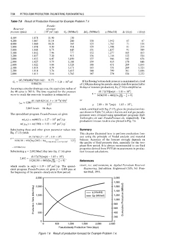
¼ 2,065 hours ¼ 86 days: which, combined with Eq. (7.17), gives the production fore-
cast shown in Table 7.6, where z-factors and real gas pseudo-
The spreadsheet program PseudoPressure.xls gives
pressures were obtained using spreadsheet programs Hall-
9
2
m( p i ) ¼ m(4613) ¼ 1:27 10 psi =cp Yarborogh-z.xls and PseudoPressure.xls, respectively. The
: production forecast result is also plotted in Fig. 7.6.
2
8
m( p wf ) ¼ m(1500) ¼ 1:85 10 psi =cp
Substituting these and other given parameter values into Summary
Eq. (7.15) yields This chapter illustrated how to perform production fore-
9
(0:17)(78)[1:27 10 1:85 10 ] 8 cast using the principle of Nodal analysis and material
q ¼
0:17
1638(180 þ 460) log (2065) þ log (0:14)(0:0251)(1:5 10 4 )(0:328) 2 3:23 balance. Accuracy of the forecast strongly depends on
the quality of fluid property data, especially for the two-
phase flow period. It is always recommended to use fluid
¼ 2,092 Mscf=day:
properties derived from PVT lab measurements in produc-
Substituting q ¼ 2,092 Mscf=day into Eq. (7.16) gives tion forecast calculations.
8
p
(0:17)(78)[m( p) 1:85 10 ]
2,092 ¼ ,
3
745
1424(180 þ 460) ln 0:328 þ 0 References
4
2
9
p
which results in m( p) ¼ 1:19 10 psi =cp. The spread- craft, b.c. and hawkins, m. Applied Petroleum Reservoir
sheet program PseudoPressure.xls gives p ¼ 4,409 psia at Engineering, 2nd edition. Englewood Cliffs, NJ: Pren-
p
the beginning of the pseudo–steady-state flow period. tice Hall, 1991.
2,500 2,000
1,800
Production Rate (Mscf/day) 1,500 q (Mscf/d) 1,200 Cumulative Production (MMscf)
1,600
2,000
1,400
Gp (MMscf)
1,000
800
1,000
600
400
500
200
0 0
0 500 1,000 1,500 2,000 2,500
Pseudosteady Production Time (days)
Figure 7.6 Result of production forecast for Example Problem 7.4.