Page 100 - Petroleum Production Engineering, A Computer-Assisted Approach

Guo, Boyun / Computer Assited Petroleum Production Engg 0750682701_chap07 Final Proof page 92 3.1.2007 8:47pm Compositor Name: SJoearun

7/92 PETROLEUM PRODUCTION ENGINEERING FUNDAMENTALS
k ro ¼ 10 (4:8455S g þ0:301) all reservoir boundaries are reached, a pseudo–steady-state
k rg ¼ 0:730678S g 1:892 flow should prevail for a volumetric gas reservoir. For a
circular reservoir, the time required for the pressure wave
Solution Example Problem 7.3 is solved using spreadsheets to reach the reservoir boundary can be estimated with
Pseudo-Steady-2PhaseProductionForecast.xls and Pseudo- t pss 1200 fmc t r e 2 .
k
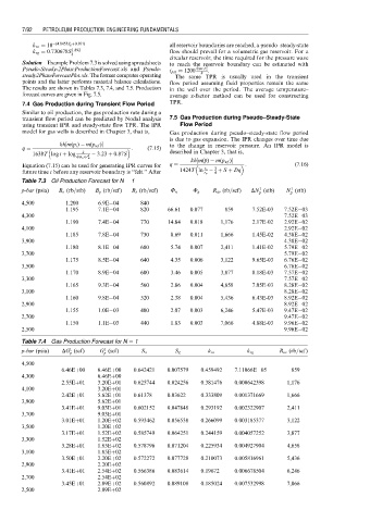
steady2PhaseForecastPlot.xls. The former computes operating The same TPR is usually used in the transient
points and the latter performs material balance calculations. flow period assuming fluid properties remain the same
The results are shown in Tables 7.3, 7.4, and 7.5. Production in the well over the period. The average temperature–
forecast curves are given in Fig. 7.5. average z-factor method can be used for constructing
7.4 Gas Production during Transient Flow Period TPR.
Similar to oil production, the gas production rate during a
transient flow period can be predicted by Nodal analysis 7.5 Gas Production during Pseudo–Steady-State
using transient IPR and steady-state flow TPR. The IPR Flow Period
model for gas wells is described in Chapter 3, that is, Gas production during pseudo–steady-state flow period
is due to gas expansion. The IPR changes over time due
kh½m(p i ) m(p wf )Š to the change in reservoir pressure. An IPR model is
q ¼ : (7:15)
k
1638T log t þ log fm o c t r 2 3:23 þ 0:87S described in Chapter 3, that is,
w kh½m( p) m(p wf )Š
p
Equation (7.15) can be used for generating IPR curves for q ¼ : (7:16)
3
future time t before any reservoir boundary is ‘‘felt.’’ After 1424T ln r e r w þ S þ Dq
4
Table 7.3 Oil Production Forecast for N ¼ 1
1
1
p-bar (psia) B o (rb=stb) B g (rb=scf) R s (rb=scf) F n F g R av (rb=scf) DN (stb) N (stb)
p p
4,500 1.200 6.9E 04 840
1.195 7.1E 04 820 66.61 0.077 859 7.52E-03 7.52E 03
4,300 7.52E 03
1.190 7.4E 04 770 14.84 0.018 1,176 2.17E-02 2.92E 02
4,100 2.92E 02
1.185 7.8E 04 730 8.69 0.011 1,666 1.45E-02 4.38E 02
3,900 4.38E 02
1.180 8.1E 04 680 5.74 0.007 2,411 1.41E-02 5.79E 02
3,700 5.79E 02
1.175 8.5E 04 640 4.35 0.006 3,122 9.65E-03 6.76E 02
3,500 6.76E 02
1.170 8.9E 04 600 3.46 0.005 3,877 8.18E-03 7.57E 02
3,300 7.57E 02
1.165 9.3E 04 560 2.86 0.004 4,658 7.05E-03 8.28E 02
3,100 8.28E 02
1.160 9.8E 04 520 2.38 0.004 5,436 6.43E-03 8.92E 02
2,900 8.92E 02
1.155 1.0E 03 480 2.07 0.003 6,246 5.47E-03 9.47E 02
2,700 9.47E 02
1.150 1.1E 03 440 1.83 0.003 7,066 4.88E-03 9.96E 02
2,500 9.96E 02
Table 7.4 Gas Production Forecast for N ¼ 1
1
1
p-bar (psia) DG (scf) G (scf) S o S g k ro k rg R av (rb=scf)
p p
4,500
6.46Eþ00 6.46Eþ00 0.642421 0.007579 0.459492 7.11066E 05 859
4,300 6.46Eþ00
2.55Eþ01 3.20Eþ01 0.625744 0.024256 0.381476 0.000642398 1,176
4,100 3.20Eþ01
2.42Eþ01 5.62Eþ01 0.61378 0.03622 0.333809 0.001371669 1,666
3,900 5.62Eþ01
3.41Eþ01 9.03Eþ01 0.602152 0.047848 0.293192 0.002322907 2,411
3,700 9.03Eþ01
3.01Eþ01 1.20Eþ02 0.593462 0.056538 0.266099 0.003185377 3,122
3,500 1.20Eþ02
3.17Eþ01 1.52Eþ02 0.585749 0.064251 0.244159 0.004057252 3,877
3,300 1.52Eþ02
3.28Eþ01 1.85Eþ02 0.578796 0.071204 0.225934 0.004927904 4,658
3,100 1.85Eþ02
3.50Eþ01 2.20Eþ02 0.572272 0.077728 0.210073 0.005816961 5,436
2,900 2.20Eþ02
3.41Eþ01 2.54Eþ02 0.566386 0.083614 0.19672 0.006678504 6,246
2,700 2.54Eþ02
3.45Eþ01 2.89Eþ02 0.560892 0.089108 0.185024 0.007532998 7,066
2,500 2.89Eþ02