Page 97 - Petroleum Production Engineering, A Computer-Assisted Approach

Guo, Boyun / Computer Assited Petroleum Production Engg 0750682701_chap07 Final Proof page 89 3.1.2007 8:47pm Compositor Name: SJoearun

FORECAST OF WELL PRODUCTION 7/89
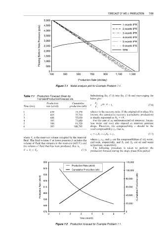
5,000 1-month IPR
4,500
Flowing Bottom Hole Pressure (psia) 3,500 4-month IPR
2-month IPR
4,000
3-month IPR
3,000
5-month IPR
6-month IPR
2,500
TPR
2,000
1,500
1,000
500
0
100 300 500 700 900 1,100 1,300

Production Rate (stb/day)
Figure 7.1 Nodal analysis plot for Example Problem 7.1.

Table 7.1 Production Forecast Given by Substituting Eq. (7.5) into Eq. (7.4) and rearranging the
TransientProductionForecast.xls latter give
Production Cumulative V p c(p i p)
p
Time (mo) rate (stb/d) production (stb) r ¼ V i ¼ e 1, (7:6)
1 639 19,170 where r is the recovery ratio. If the original oil in place N is
2 618 37,710 known, the cumulative recovery (cumulative production)
3 604 55,830 is simply expressed as N p ¼ rN.
4 595 73,680 For the case of an undersaturated oil reservoir, forma-
5 588 91,320 tion water and rock also expand as reservoir pressure
6 583 108,795 drops. Therefore, the compressibility c should be the
total compressibility c t , that is,
c t ¼ c o S o þ c w S w þ c f , (7:7)
where V i is the reservoir volume occupied by the reservoir
p
fluid. The fluid volume V at lower pressure p includes the where c o , c w , and c f are the compressibilities of oil, water,
volume of fluid that remains in the reservoir (still V i ) and and rock, respectively, and S o and S w are oil and water
the volume of fluid that has been produced, that is, saturations, respectively.
The following procedure is taken to perform the
V ¼ V i þ V p : (7:5) production forecast during the single-phase flow period:

650 120,000
Production Rate (stb/d)
640
Cumulative Production (stb) 100,000
630 80,000
Production Rate (stb/d) 610 60,000 Cumulative Production (stb)
620

600
590 40,000
20,000
580
570 0
0 1 2 3 4 5 6 7
Time (month)

Figure 7.2 Production forecast for Example Problem 7.1.