Page 99 - Petroleum Production Engineering, A Computer-Assisted Approach

Guo, Boyun / Computer Assited Petroleum Production Engg 0750682701_chap07 Final Proof page 91 3.1.2007 8:47pm Compositor Name: SJoearun

FORECAST OF WELL PRODUCTION 7/91
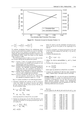
600 1.E+06

1.E+06
500 1.E+06
Production Rate (stb/day) 300 8.E+05 Cumulative Production (stb)
400

6.E+05
200

100 Production Rate 4.E+05
2.E+05
Cumulative Production
0 0.E+00
0 500 1,000 1,500 2,000 2,500
Pseudosteady State Production Time (days)
Figure 7.4 Production forecast for Example Problem 7.2.

" #

1
1
J p p p wf p wf 2 where N and G are the cumulative oil and gas pro-
q ¼ 1 0:2 0:8 : (7:8) p p
1:8 p p p p duction per stb of oil in place at the beginning of the
interval.
To perform production forecast for solution-gas drive 3. Calculate cumulative oil and gas production at the end
1
reservoirs, material balance models are used for establish- of the interval by adding DN and DG to N and G ,
1
1
1
ing the relation of the cumulative production to time. The respectively. p p p p
commonly used material balance model is found in Craft 4. Calculate oil saturation by
and Hawkins (1991), which was based on the original
work of Tarner (1944). B o 1
The following procedure is taken to carry out a produc- S o ¼ (1 S w )(1 N ): (7:13)
p
B oi
tion forecast during the two-phase flow period:
5. Obtain the relative permeabilities k rg and k ro based
Step 1: Assume a series of average-reservoir pressure p ¯ on S o .
values between the bubble-point pressure p b and 6. Calculate the average gas–oil ratio by
abandonment reservoir pressure p a .
Step 2: Estimate fluid properties at each average-reservoir R R ¼ R s þ k rg m o B o , (7:14)
pressure, and calculate incremental cumulative k ro m g B g
production DN p and cumulative production N p
within each average-reservoir pressure interval. where again B g should be in rb/scf if R s is in scf/stb.
Step 3: Perform Nodal analyses to estimate production 7. Compare the calculated R with the value assumed in
R
rate q at each average-reservoir pressure. Step 2. Repeat Steps 2 through 6 until R converges.
R
Step 4: Calculate production time Dt for each average-
reservoir pressure interval by Dt ¼ DN p =q and Example Problem 7.3 For the oil reservoir described in
P
the cumulative production time by t ¼ Dt.
Example Problem 7.2, predict the oil production rate and
Step 2 is further described in the following procedure: cumulative oil production over the time interval during
which reservoir pressure declines from bubble-point
1. Calculate coefficients F n and F g for the two pressure pressure to abandonment reservoir pressure of 2,500. The
values that define the pressure interval, and obtain following additional data are given:

F
F
average values F n and F g in the interval. The F n and
F g are calculated using
B o R s B g
F n ¼ , (7:9) Reservoir
(B o B oi ) þ (R si R s )B g pressure (psia) B o (rb /stb) B g (rb /scf) R s (rb /scf) m g (cp)
B g
F g ¼ , (7:10)
(B o B oi ) þ (R si R s )B g 4,500 1.200 6.90E 04 840 0.01
where B g should be in rb/scf if R s is in scf/stb. 4,300 1.195 7.10E 04 820 0.01
4,100 1.190 7.40E 04 770 0.01
2. Assume an average gas–oil ratio R ¯ in the interval, and 3,900 1.185 7.80E 04 730 0.01
calculate incremental oil and gas production per stb of 3,700 1.180 8.10E 04 680 0.01
oil in place by 3,500 1.175 8.50E 04 640 0.01
3,300 1.170 8.90E 04 600 0.01

1
1 F n N F g G 1 p 3,100 1.165 9.30E 04 560 0.01
F
F
p
1
DN ¼ , (7:11) 2,900 1.160 9.80E 04 520 0.01
p
F
R
F F n þ RF g
2,700 1.155 1.00E 03 480 0.01
1
1
R
DG ¼ DN R, (7:12) 2,500 1.150 1.10E 03 440 0.01
p
p