Page 143 - Petroleum Production Engineering, A Computer-Assisted Approach

Guo, Boyun / Computer Assited Petroleum Production Engg 0750682701_chap11 Final Proof page 138 3.1.2007 8:54pm Compositor Name: SJoearun

11/138 EQUIPMENT DESIGN AND SELECTION
11.3.2 Reciprocating Compressors Pv ¼ RT (11:33)
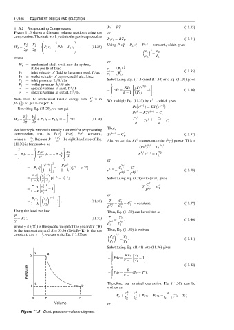
Figure 11.5 shows a diagram volume relation during gas or
compression. The shaft work put into the gas is expressed as
0 1 P 1 v 1 ¼ RT 1 : (11:34)
k
k
V 2 V 2 ð 2 Using P 1 n ¼ P 2 n ¼ Pn ¼ constant, which gives
k
A
W s ¼ 2 1 þ @ P 2 v 2 Pdv P 1 v 1 , (11:29) 1 2
2g 2g k
v 1 P 2
1 ¼
where v 2 P 1
or
W s ¼ mechanical shaft work into the system,
ft-lbs per lb of fluid v 1 P 2 1 k
V 1 ¼ inlet velocity of fluid to be compressed, ft/sec ¼ : (11:35)
v 2 P 1
V 2 ¼ outlet velocity of compressed fluid, ft/sec
2
P 1 ¼ inlet pressure, lb=ft abs Substituting Eqs. (11.35) and (11.34) into Eq. (11.31) gives
2
P 2 ¼ outlet pressure, lb=ft abs ð 2 " k 1 #
3
n 1 ¼ specific volume at inlet, ft =lb Pdv ¼ RT 1 P 2 k 1 : (11:36)
3
n 2 ¼ specific volume at outlet, ft =lb. k 1 P 1
1
Note that the mechanical kinetic energy term V 2g 2 is in We multiply Eq. (11.33) by n k 1 , which gives

ft lb to get ft-lbs per lb.
lb k 1 k 1
Rewriting Eq. (11.29), we can get Pv v ¼ RT v
k
Pv ¼ RTv k 1
ð 2 ¼ C 1
V 2 V 2 k
W s þ 1 2 þ P 1 v 1 P 2 v 2 ¼ Pdv: (11:30) Pv k 1 C 1 0
2g 2g ¼ Tv ¼ ¼ C 1
1 R R
Thus,
An isentropic process is usually assumed for reciprocating
k
k
k
compression, that is, P 1 n ¼ P 2 n ¼ Pn ¼ constant, Tv k 1 ¼ C : 0 (11:37)
1
2
1
P 1 v k
where k ¼ . Because P ¼ v k , the right-hand side of Eq. k k 1
c p
1
c v Also we can rise Pv ¼ constant to the k power. This is
(11.30) is formulated as
k k 1 0 k 1
(Pv ) k ¼ C 1 k
ð 2 ð 2 ð 2
P 1 v k dv k 1 k 1 0k 1
Pdv ¼ 1 dv ¼ P 1 v k P k v ¼ C 1 k
v k 1 v k
1 1 1 or
1 k 2 k 0 k 1
¼ P 1 v k v ¼ P 1 v 1 [v 1 k v 1 k ] C k C 00
1
1
1 k 1 k 2 1 n k 1 ¼ 1 k 1 ¼ k 1 : (11:38)
1 P k P k
P 1 v k v 1 k
¼ 1 1 [v 1 k v 1 k ] Substituting Eq. (3.38) into (3.37) gives
1
2
1 k v 1 k
1
C 00
P 1 v 1 v 1 k T 1 0
¼ 2 1 k 1 ¼ C 1
1 k v 1 k P k
1
" # or
k 1
P 1 v 1 v 1 0
¼ 1 : (11:31) T C 000
1 k v 2 k 1 ¼ 1 00 ¼ C ¼ constant: (11:39)
1
P k C 1
Using the ideal gas law
Thus, Eq. (11.39) can be written as
P
¼ RT, (11:32) T 1 T 2
g k 1 ¼ k 1 : (11:40)
P 1 k P 2 k
3
where g (lb=ft ) is the specific weight of the gas and T (8R)
is the temperature and R ¼ 53:36 (lb-ft/lb-8R) is the gas Thus, Eq. (11.40) is written
1
constant, and v ¼ , we can write Eq. (11.32) as k 1
g P 2 k T 2
¼ : (11:41)
P 1 T 1
Substituting Eq. (11.41) into (11.36) gives
d ð 2
2 c RT 1 T 2
Pdv ¼ 1
k 1 T 1
1 ð 2 (11:42)
Pressure Pdv ¼ k 1 (T 2 T 1 ):
R
1
a Therefore, our original expression, Eq. (11.30), can be
1 b
written as
V 2 V 2 R
W s þ 1 2 þ P 1 v 1 P 2 v 2 ¼ (T 2 T 1 )
o m n 2g 2g k 1
Volume or
Figure 11.5 Basic pressure–volume diagram.