Page 188 - Petroleum Production Engineering, A Computer-Assisted Approach

Guo, Boyun / Computer Assited Petroleum Production Engg 0750682701_chap13 Final Proof page 184 3.1.2007 9:07pm Compositor Name: SJoearun

13/184 ARTIFICIAL LIFT METHODS

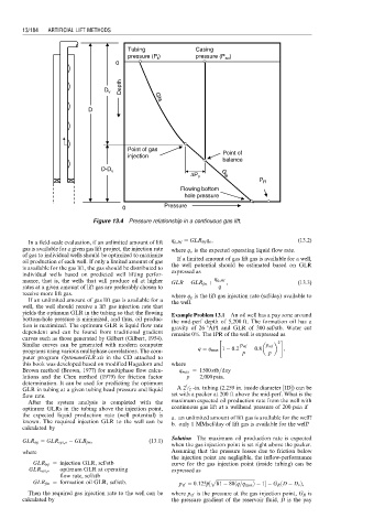
Tubing Casing
pressure (P ) t pressure (P )
so
0

Depth
D v Gfa

D

Point of gas
Point of
injection
balance
D-D v
∆P v G fb
P R
Flowing bottom
hole pressure
Pressure
0
Figure 13.4 Pressure relationship in a continuous gas lift.

In a field-scale evaluation, if an unlimited amount of lift q g,inj ¼ GLR inj q o , (13:2)
gas is available for a given gas lift project, the injection rate where q o is the expected operating liquid flow rate.
of gas to individual wells should be optimized to maximize
oil production of each well. If only a limited amount of gas If a limited amount of gas lift gas is available for a well,
is available for the gas lift, the gas should be distributed to the well potential should be estimated based on GLR
individual wells based on predicted well lifting perfor- expressed as
mance, that is, the wells that will produce oil at higher GLR ¼ GLR fm þ q g,inj , (13:3)
rates at a given amount of lift gas are preferably chosen to q
receive more lift gas. where q g is the lift gas injection rate (scf/day) available to
If an unlimited amount of gas lift gas is available for a the well.
well, the well should receive a lift gas injection rate that
yields the optimum GLR in the tubing so that the flowing Example Problem 13.1 An oil well has a pay zone around
bottom-hole pressure is minimized, and thus, oil produc- the mid-perf depth of 5,200 ft. The formation oil has a
tion is maximized. The optimum GLR is liquid flow rate gravity of 26 8API and GLR of 300 scf/stb. Water cut
dependent and can be found from traditional gradient remains 0%. The IPR of the well is expressed as
curves such as those generated by Gilbert (Gilbert, 1954). " #
Similar curves can be generated with modern computer p wf p wf 2
programs using various multiphase correlations. The com- q ¼ q max 1 0:2 p p 0:8 p p ,
puter program OptimumGLR.xls in the CD attached to
this book was developed based on modified Hagedorn and where
Brown method (Brown, 1977) for multiphase flow calcu- q max ¼ 1500 stb=day
lations and the Chen method (1979) for friction factor p p ¼ 2,000 psia.
determination. It can be used for predicting the optimum 1
GLR in tubing at a given tubing head pressure and liquid A2 ⁄ 2 -in. tubing (2.259 in. inside diameter [ID]) can be
flow rate. set with a packer at 200 ft above the mid-perf. What is the
After the system analysis is completed with the maximum expected oil production rate from the well with
optimum GLRs in the tubing above the injection point, continuous gas lift at a wellhead pressure of 200 psia if
the expected liquid production rate (well potential) is a. an unlimited amount of lift gas is available for the well?
known. The required injection GLR to the well can be b. only 1 MMscf/day of lift gas is available for the well?
calculated by
Solution The maximum oil production rate is expected
GLR inj ¼ GLR opt,o GLR fm , (13:1)
when the gas injection point is set right above the packer.
where Assuming that the pressure losses due to friction below
the injection point are negligible, the inflow-performance
GLR inj ¼ injection GLR, scf/stb curve for the gas injection point (inside tubing) can be
GLR opt,o ¼ optimum GLR at operating expressed as
flow rate, scf/stb p ffiffiffiffiffiffiffiffiffiffiffiffiffiffiffiffiffiffiffiffiffiffiffiffiffiffiffiffiffiffiffiffiffi
GLR fm ¼ formation oil GLR, scf/stb. p vf ¼ 0:125 p½ 81 80 q=q max Þ 1Š G R D D v Þ,
ð
p
ð
Then the required gas injection rate to the well can be where p vf is the pressure at the gas injection point, G R is
calculated by the pressure gradient of the reservoir fluid, D is the pay