Page 64 - Petroleum Production Engineering, A Computer-Assisted Approach

Guo, Boyun / Petroleum Production Engineering, A Computer-Assisted Approach 0750682701_chap04 Final Proof page 55 22.12.2006 6:07pm

WELLBORE PERFORMANCE 4/55
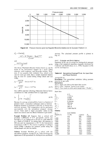
Pressure (psia)
0 500 1,000 1,500 2,000 2,500 3,000 3,500
0

2,000

4,000
Depth (ft) 6,000

8,000

10,000

12,000
Figure 4.4 Pressure traverse given by HagedornBrownCorrelation.xls for Example Problem 4.4.

p 2 ¼ Exp(s)p 2 sections. The calculated pressure profile is plotted in
wf hf
2
2
4
z
6:67 10 [Exp(s) 1]f M q z T 2 Fig. 4.5.
T
þ sc (4:54)
5
d cos u
i
and 4.4.2 Cullender and Smith Method
Equation (4.50) can be solved for bottom-hole pressure
0:0375g g L cos u
s ¼ (4:55) using a fast numerical algorithm originally developed by
z Cullender and Smith (Katz et al., 1959). Equation (4.50)
zT
T
The Darcy–Wiesbach (Moody) friction factor f M can be can be rearranged as
found in the conventional manner for a given tubing
diameter, wall roughness, and Reynolds number. How-
ever, if one assumes fully turbulent flow, which is the Table 4.4 Spreadsheet AverageTZ.xls: the Input Data
case for most gas wells, then a simple empirical relation and Result Sections
may be used for typical tubing strings (Katz and Lee
1990): AverageTZ.xls
Description: This spreadsheet calculates tubing pressure
0:01750
f M ¼ for d i # 4:277 in: (4:56) traverse for gas wells.
d i 0:224 Instructions:
Step 1: Input your data in the Input data section.
0:01603 Step 2: Click ‘‘Solution’’ button to get results.
f M ¼ for d i > 4:277 in: (4:57)
d i 0:164 Step 3: View results in table and in graph sheet ‘‘Profile’’.
Guo (2001) used the following Nikuradse friction factor Input data
correlation for fully turbulent flow in rough pipes:
2 3 2 g g ¼ 0.71
1 d ¼ 2.259 in.
f M ¼ 4 5 (4:58) «=d ¼ 0.0006
1:74 2 log 2«
d i L ¼ 10.000 ft
u ¼ 0 degrees
Because the average compressibility factor is a function of
pressure itself, a numerical technique such as Newton– p hf ¼ 800 psia
Raphson iteration is required to solve Eq. (4.54) for bot- T hf ¼ 150 8F
tom-hole pressure. This computation can be performed T wf ¼ 200 8F
automatically with the spreadsheet program Average q sc ¼ 2,000 Mscf/d
TZ.xls. Users need to input parameter values in the Solution
Input data section and run Macro Solution to get results. f M ¼ 0.017396984
Depth (ft) T (8R) p (psia) Z av
Example Problem 4.5 Suppose that a vertical well 0 610 800 0.9028
produces 2 MMscf/d of 0.71 gas-specific gravity gas 1,000 615 827 0.9028
7
through a 2 ⁄ 8 in. tubing set to the top of a gas reservoir 2,000 620 854 0.9027
at a depth of 10,000 ft. At tubing head, the pressure is 3,000 625 881 0.9027
800 psia and the temperature is 150 8F; the bottom-hole 4,000 630 909 0.9026
temperature is 200 8F. The relative roughness of tubing is 5,000 635 937 0.9026
about 0.0006. Calculate the pressure profile along the 6,000 640 965 0.9026
tubing length and plot the results. 7,000 645 994 0.9026
8,000 650 1023 0.9027
Solution Example Problem 4.5 is solved with the 9,000 655 1053 0.9027
spreadsheet program AverageTZ.xls. Table 4.4 shows the 10,000 660 1082 0.9028
appearance of the spreadsheet for the Input data and Result