Page 60 - Petroleum Production Engineering, A Computer-Assisted Approach

Guo, Boyun / Petroleum Production Engineering, A Computer-Assisted Approach 0750682701_chap04 Final Proof page 51 22.12.2006 6:07pm

WELLBORE PERFORMANCE 4/51
Based on comprehensive comparisons of these models,
Total measured depth: 7,000 ft Ansari et al. (1994) and Hasan and Kabir (2002) recom-
The average inclination angle: 20 deg mended the Hagedorn–Brown method with modifications
Tubing inner diameter: 1.995 in. for near-vertical flow.
Gas production rate: 1 MMscfd The modified Hagedorn–Brown (mH-B) method is an
Gas-specific gravity: 0.7 air ¼ 1 empirical correlation developed on the basis of the original
Oil production rate: 1,000 stb/d work of Hagedorn and Brown (1965). The modifications
Oil-specific gravity: 0.85 H 2 O ¼ 1 include using the no-slip liquid holdup when the original
Water production rate: 300 bbl/d correlation predicts a liquid holdup value less than the no-
Water-specific gravity: 1.05 H 2 O ¼ 1 slip holdup and using the Griffith correlation (Griffith and
3
Solid production rate: 1 ft =d Wallis, 1961) for the bubble flow regime.
Solid specific gravity: 2.65 H 2 O ¼ 1 The original Hagedorn–Brown correlation takes the fol-
Tubing head temperature: 100 8F lowing form:
Bottom hole temperature: 224 8F
Tubing head pressure: 300 psia dP g 2f F u 2 D(u )
2
r
r
¼ r r þ m þ r r m , (4:26)
dz g c g c D 2g c Dz
Solution This example problem is solved with the which can be expressed in U.S. field units as
spreadsheet program Guo-GhalamborBHP.xls. The result
is shown in Table 4.2.
2
dp f F M 2 D(u )
r
r
144 ¼ þ t þ r r m , (4:27)
5
10
dz 7:413 10 D 2g c Dz
r
r
4.3.3.2 Separated-Flow Models
A number of separated-flow models are available for TPR where
calculations. Among many others are the Lockhart and
Martinelli correlation (1949), the Duns and Ros correla- M t ¼ total mass flow rate, lb m =d
tion (1963), and the Hagedorn and Brown method (1965). r r ¼ in situ average density, lb m =ft 3
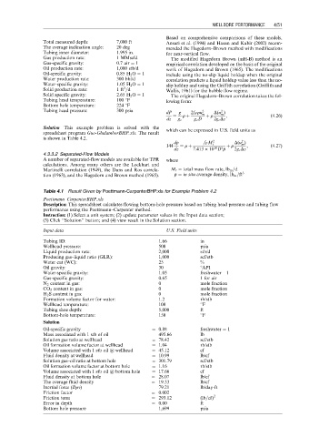
Table 4.1 Result Given by Poettmann-CarpenterBHP.xls for Example Problem 4.2
Poettmann–CarpenterBHP.xls
Description: This spreadsheet calculates flowing bottom-hole pressure based on tubing head pressure and tubing flow
performance using the Poettmann–Carpenter method.
Instruction: (1) Select a unit system; (2) update parameter values in the Input data section;
(3) Click ‘‘Solution’’ button; and (4) view result in the Solution section.
Input data U.S. Field units
Tubing ID: 1.66 in
Wellhead pressure: 500 psia
Liquid production rate: 2,000 stb/d
Producing gas–liquid ratio (GLR): 1,000 scf/stb
Water cut (WC): 25 %
Oil gravity: 30 8API
Water-specific gravity: 1.05 freshwater ¼1
Gas-specific gravity: 0.65 1 for air
N 2 content in gas: 0 mole fraction
CO 2 content in gas: 0 mole fraction
H 2 S content in gas: 0 mole fraction
Formation volume factor for water: 1.2 rb/stb
Wellhead temperature: 100 8F
Tubing shoe depth: 5,000 ft
Bottom-hole temperature: 150 8F
Solution
Oil-specific gravity ¼ 0.88 freshwater ¼ 1
Mass associated with 1 stb of oil ¼ 495.66 lb
Solution gas ratio at wellhead ¼ 78.42 scf/stb
Oil formation volume factor at wellhead ¼ 1.04 rb/stb
Volume associated with 1 stb oil @ wellhead ¼ 45.12 cf
Fluid density at wellhead ¼ 10.99 lb/cf
Solution gas–oil ratio at bottom hole ¼ 301.79 scf/stb
Oil formation volume factor at bottom hole ¼ 1.16 rb/stb
Volume associated with 1 stb oil @ bottom hole ¼ 17.66 cf
Fluid density at bottom hole ¼ 28.07 lb/cf
The average fluid density ¼ 19.53 lb/cf
Inertial force (Drv) ¼ 79.21 lb/day-ft
Friction factor ¼ 0.002
Friction term ¼ 293.12 (lb=cf) 2
Error in depth ¼ 0.00 ft
Bottom hole pressure ¼ 1,699 psia