Page 65 - Petroleum Production Engineering, A Computer-Assisted Approach

Guo, Boyun / Petroleum Production Engineering, A Computer-Assisted Approach 0750682701_chap04 Final Proof page 56 22.12.2006 6:07pm

4/56 PETROLEUM PRODUCTION ENGINEERING FUNDAMENTALS
Pressure (psia)
0 200 400 600 800 1,000 1,200
0
1,000
2,000
3,000

4,000
Depth (ft) 5,000

6,000
7,000
8,000
9,000
10,000

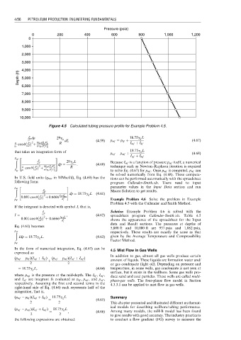
Figure 4.5 Calculated tubing pressure profile for Example Problem 4.5.

P dp 29g g 18:75g g L
zT
8f M Q 2 P 2 ¼ dL (4:59) p mf ¼ p hf þ (4:67)
g P 2 R I mf þ I hf
cos u þ sc sc
g c zT p 2 g c D 5 T 2
i sc
that takes an integration form of p wf ¼ p mf þ 18:75g g L (4:68)
2 3 I wf þ I mf
P
ð wf P 29g g L
4 zT 5 : (4:60) Because I mf is a function of pressure p mf itself, a numerical
g P 2 8f M Q 2 P 2 dp ¼ R technique such as Newton–Raphson iteration is required
cos u þ sc sc
P hf g c zT p 2 g c D 5 T 2 sc to solve Eq. (4.67) for p mf . Once p mf is computed, p wf can
i
be solved numerically from Eq. (4.68). These computa-
In U.S. field units (q msc in MMscf/d), Eq. (4.60) has the tions can be performed automatically with the spreadsheet
following form: program Cullender-Smith.xls. Users need to input
2 3 parameter values in the Input Data section and run
p ð wf p
4 zT 5 dp ¼ 18:75g g L (4:61) Macro Solution to get results.
0:001 cos u p 2 þ 0:6666 f M q 2 msc
p hf zT d 5 i Example Problem 4.6 Solve the problem in Example
Problem 4.5 with the Cullender and Smith Method.
If the integrant is denoted with symbol I, that is,
p Solution Example Problem 4.6 is solved with the
I ¼ zT f M q 2 , (4:62) spreadsheet program Cullender-Smith.xls. Table 4.5
p 2
0:001 cos u zT þ 0:6666 d 5 sc shows the appearance of the spreadsheet for the Input
i
data and Result sections. The pressures at depths of
Eq. (4.61) becomes
5,000 ft and 10,000 ft are 937 psia and 1,082 psia,
p
ð wf respectively. These results are exactly the same as that
Idp ¼ 18:75g g L: (4:63) given by the Average Temperature and Compressibility
Factor Method.
p hf
In the form of numerical integration, Eq. (4.63) can be 4.5 Mist Flow in Gas Wells
expressed as
In addition to gas, almost all gas wells produce certain
(p mf p hf )(I mf þ I hf ) (p wf p mf )(I wf þ I mf )
þ amount of liquids. These liquids are formation water and/
2 2 or gas condensate (light oil). Depending on pressure and
¼ 18:75g g L, (4:64) temperature, in some wells, gas condensate is not seen at
surface, but it exists in the wellbore. Some gas wells pro-
where p mf is the pressure at the mid-depth. The I hf , I mf , duce sand and coal particles. These wells are called multi-
and I wf are integrant Is evaluated at p hf , p mf , and p wf , phase-gas wells. The four-phase flow model in Section
respectively. Assuming the first and second terms in the 4.3.3.1 can be applied to mist flow in gas wells.
right-hand side of Eq. (4.64) each represents half of the
integration, that is,
(p mf p hf )(I mf þ I hf ) 18:75g g L Summary
¼ (4:65)
2 2 This chapter presented and illustrated different mathemat-
ical models for describing wellbore/tubing performance.
(p wf p mf )(I wf þ I mf ) 18:75g g L
¼ , (4:66) Among many models, the mH-B model has been found
2 2 to give results with good accuracy. The industry practice is
the following expressions are obtained: to conduct a flow gradient (FG) survey to measure the