Page 73 - Petroleum Production Engineering, A Computer-Assisted Approach

Guo, Boyun / Petroleum Production Engineering, A Computer-Assisted Approach 0750682701_chap05 Final Proof page 64 21.12.2006 2:02pm

5/64 PETROLEUM PRODUCTION ENGINEERING FUNDAMENTALS
Table 5.2 Solution Given by the Spreadsheet Program 5.5.2 Subcritical (Subsonic) Flow
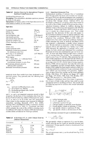
GasDownChokePressure.xls Mathematical modeling of subsonic flow of multiphase
fluid through choke has been controversial over decades.
GasDownChokePressure.xls Fortunati (1972) was the first investigator who presented a
Description: This spreadsheet calculates upstream pressure model that can be used to calculate critical and subcritical
at choke for dry gases. two-phase flow through chokes. Ashford (1974) also
Instructions: (1) Update values in the Input data section; (2)
click Solution button; (3) view results. developed a relation for two-phase critical flow based on
the work of Ros (1960). Gould (1974) plotted the critical–
subcritical boundary defined by Ashford, showing that
Input data
different values of the polytropic exponents yield different
boundaries. Ashford and Pierce (1975) derived an equa-
Upstream pressure: 700 psia
1
Choke size: 32 ⁄ 64 in. tion to predict the critical pressure ratio. Their model
Flowline ID: 2 in. assumes that the derivative of flow rate with respect to
Gas production rate: 2,500 Mscf/d the downstream pressure is zero at critical conditions. One
Gas-specific gravity: 0.75 1 for air set of equations was recommended for both critical and
Gas-specific heat ratio (k): 1.3 subcritical flow conditions. Pilehvari (1980, 1981) also
Upstream temperature: 110 8F studied choke flow under subcritical conditions. Sachdeva
Choke discharge coefficient: 0.99 (1986) extended the work of Ashford and Pierce (1975)
and proposed a relationship to predict critical pressure
Solution ratio. He also derived an expression to find the boundary
Choke area: 0.19625 in: 2 between critical and subcritical flow. Surbey et al. (1988,
Critical pressure ratio: 0.5457 1989) discussed the application of multiple orifice valve
Minimum downstream pressure 382 psia chokes for both critical and subcritical flow conditions.
for minimum sonic flow: Empirical relations were developed for gas and water sys-
Flow rate at the minimum 3,857 Mscf/d tems. Al-Attar and Abdul-Majeed (1988) made a compari-
sonic flow condition: son of existing choke flow models. The comparison was
Flow regime 1 based on data from 155 well tests. They indicated that the
(1 ¼ sonic flow; 1 ¼ subsonic flow): best overall comparison was obtained with the Gilbert cor-
The maximum possible 382 psia relation, which predicted measured production rate within
downstream pressure in sonic flow: an average error of 6.19%. On the basis of energy equation,
Downstream pressure given by 626 psia Perkins (1990) derived equations that describe isentropic
subsonic flow equation: flow of multiphase mixtures through chokes. Osman and
Estimated downstream pressure: 626 psia Dokla (1990) applied the least-square method to field data
to develop empirical correlations for gas condensate choke
flow. Gilbert-type relationships were generated. Applica-
tions of these choke flow models can be found elsewhere
empirical choke flow models have been developed in the (Wallis, 1969; Perry, 1973; Brown and Beggs, 1977; Brill
past half century. They generally take the following form and Beggs, 1978; Ikoku, 1980; Nind, 1981; Bradley, 1987;
for sonic flow: Beggs, 1991; Rastion et al., 1992; Saberi, 1996).
Sachdeva’s multiphase choke flow mode is representa-
m
CR q
p wh ¼ , (5:12) tive of most of these works and has been coded in some
S n commercial network modeling software. This model uses
where the following equation to calculate the critical–subcritical
boundary:
p wh ¼ upstream (wellhead) pressure, psia
q ¼ gross liquid rate, bbl/day 8 9 k
=
<
R ¼ producing gas-liquid ratio, Scf/bbl > k þ (1 x 1 )V L (1 y c ) > k 1
1
S ¼ choke size, ⁄ 64 in. y c ¼ k 1 x 1 V G1 h i 2 , (5:13)
> k n n (1 x 1 )V L ;
>
:
and C, m, and n are empirical constants related to fluid k 1 þ þ n(1 x 1 )V L þ 2 x 1 V G2
2
x 1 V G2
properties. On the basis of the production data from Ten
Section Field in California, Gilbert (1954) found the values where
for C, m, and n to be 10, 0.546, and 1.89, respectively. y c ¼ critical pressure ratio
Other values for the constants were proposed by different k ¼ C p =C v , specific heat ratio
researchers including Baxendell (1957), Ros (1960), n ¼ polytropic exponent for gas
Achong (1961), and Pilehvari (1980). A summary of these x 1 ¼ free gas quality at upstream, mass fraction
3
values is presented in Table 5.3. Poettmann and Beck V L ¼ liquid specific volume at upstream, ft =lbm
3
(1963) extended the work of Ros (1960) to develop charts V G1 ¼ gas specific volume at upstream, ft =lbm
3
for different API crude oils. Omana (1969) derived dimen- V G2 ¼ gas specific volume at downstream, ft =lbm.
sionless choke correlations for water-gas systems.
The polytropic exponent for gas is calculated using
x 1 (C p C v )
Table 5.3 A Summary of C, m, and n Values Given by n ¼ 1 þ : (5:14)
x 1 C v þ (1 x 1 )C L
Different Researchers
The gas-specific volume at upstream (V G1 ) can be deter-
Correlation C m n
mined using the gas law based on upstream pressure and
Gilbert 10 0.546 1.89 temperature. The gas-specific volume at downstream (V G2 )
Ros 17.4 0.5 2 is expressed as
Baxendell 9.56 0.546 1.93 V G2 ¼ V G1 y c : 1 (5:15)
k
Achong 3.82 0.65 1.88
Pilehvari 46.67 0.313 2.11 The critical pressure ratio y c can be solved from Eq. (5.13)
numerically.