Page 79 - Petroleum Production Engineering, A Computer-Assisted Approach

Guo, Boyun / Computer Assited Petroleum Production Engg 0750682701_chap06 Final Proof page 71 3.1.2007 8:40pm Compositor Name: SJoearun

WELL DELIVERABILITY 6/71
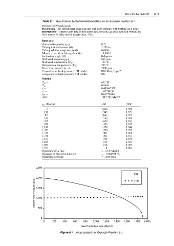
Table 6.1 Result Given by BottomHoleNodalGas.xls for Example Problem 6.1
BottomHoleNodalGas.xls
Description: This spreadsheet calculates gas well deliverability with bottom-hole node.
Instructions: (1) Input your data in the Input data section; (2) click Solution button; (3)
view results in table and in graph sheet ‘‘Plot.’’
Input data
Gas-specific gravity (g g ): 0.71
Tubing inside diameter (D): 2.259 in.
Tubing relative roughness (e/D): 0.0006
Measured depth at tubing shoe (L): 10,000 ft
Inclination angle (Q): 0 degrees
Wellhead pressure (p hf ): 800 psia
Wellhead temperature (T hf ): 150 8F
Bottom-hole temperature (T wf ): 200 8F
Reservoir pressure (p ): 2000 psia
C-constant in back-pressure IPR model: 0:01 Mscf=d-psi 2n
n-exponent in back-pressure IPR model: 0.8
Solution
T av ¼ 635 8R
Z av ¼ 0.8626
s ¼ 0.486062358
s
e ¼ 1.62590138
f M ¼ 0.017396984
AOF ¼ 1912.705 Mscf/d
q sc (Mscf/d) IPR TPR
0 2,000 1,020
191 1,943 1,021
383 1,861 1,023
574 1,764 1,026
765 1,652 1,031
956 1,523 1,037
1,148 1,374 1,044
1,339 1,200 1,052
1,530 987 1,062
1,721 703 1,073
1,817 498 1,078
1,865 353 1,081
1,889 250 1,083
1,913 0 1,084
Operating flow rate ¼ 1,470 Mscf/d
Residual of objective function ¼ 0.000940747
Operating pressure ¼ 1,059 psia

2,500
IPR
2,000
Bottom Hole Pressure (psia) 1,500
TPR

1,000

500

0
0 200 400 600 800 1,000 1,200 1,400 1,600 1,800 2,000
Gas Production Rate (Mscf/d)
Figure 6.1 Nodal analysis for Example Problem 6.1.