Page 82 - Petroleum Production Engineering, A Computer-Assisted Approach

Guo, Boyun / Computer Assited Petroleum Production Engg 0750682701_chap06 Final Proof page 74 3.1.2007 8:40pm Compositor Name: SJoearun

6/74 PETROLEUM PRODUCTION ENGINEERING FUNDAMENTALS
q. This computation can be performed automatically with performance relationship’’ (WPR), which is obtained by
the spreadsheet program BottomHoleNodalOil-HB.xls. transforming the IPR to wellhead through the TPR.
The outflow performance curve is the wellhead choke
Example Problem 6.4 For the data given in the following performance relationship (CPR). Some TPR models are
table, predict the operating point: presented in Chapter 4. CPR models are discussed in
Chapter 5.
Depth: 9,850 ft Nodal analysis with wellhead being a solution node
Tubing inner diameter: 1.995 in. is carried out by plotting the WPR and CPR curves and
Oil gravity: 45 8API finding the solution at the intersection point of the two
Oil viscosity: 2 cp curves. Again, with modern computer technologies, the solu-
Production GLR: 500 scf/bbl tion can be computed quickly without plotting the curves,
Gas-specific gravity: 0.7 air ¼ 1 although the curves are still plotted for verification.
Flowing tubing head pressure: 450 psia
Flowing tubing head temperature: 80 8F
Flowing temperature at tubing shoe: 180 8F 6.2.2.1 Gas Well
Water cut: 10% If the IPR of a well is defined by Eq. (6.1) and the TPR is
Reservoir pressure: 5,000 psia represented by Eq. (6.2), substituting Eq. (6.2) into
Bubble-point pressure: 4,000 psia Eq. (6.1) gives

Productivity index above bubble point: 1.5 stb/d-psi
2
p
q sc ¼ C p Exp(s)p 2
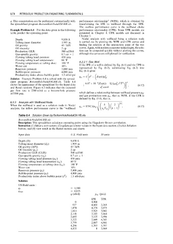
Solution Example Problem 6.4 is solved with the spread- hf
sheet program BottomHoleNodalOil-HB.xls. Table 6.4 4 2 2 2 n
T
z
sc
shows the appearance of the spreadsheet for the Input data þ 6:67 10 [Exp(s) 1] f M q z T , (6:12)
5
and Result sections. Figure 6.2 indicates that the expected d cos u
i
gas flow rate is 2200 stb/d at a bottom-hole pressure
of 3500 psia. which defines a relationship between wellhead pressure p hf
and gas production rate q sc , that is, WPR. If the CPR is
defined by Eq. (5.8), that is,
v ffiffiffiffiffiffiffiffiffiffiffiffiffiffiffiffiffiffiffiffiffiffiffiffiffiffiffiffiffiffiffiffiffiffiffiffiffiffiffiffiffiffi
6.2.2 Analysis with Wellhead Node u ! kþ1
u
When the wellhead is used as a solution node in Nodal t k 2 k 1
q sc ¼ 879CAp hf , (6:13)
analysis, the inflow performance curve is the ‘‘wellhead g g T up k þ 1
Table 6.4 Solution Given by BottomHoleNodalOil-HB.xls
BottomHoleNodalOil-HB.xls
Description: This spreadsheet calculates operating point using the Hagedorn–Brown correlation.
Instruction: (1) Select a unit system; (2) update parameter values in the Input data section; (3) click Solution
button; and (4) view result in the Result section and charts.
Input data U.S. Field units SI units
Depth (D): 9,850 ft
Tubing inner diameter (d ti ): 1.995 in.
Oil gravity (API): 45 8API
Oil viscosity (m o ): 2 cp
Production GLR (GLR): 500 scf/bbl
Gas-specific gravity (g g ): 0.7 air ¼ 1
Flowing tubing head pressure (p hf ): 450 psia
Flowing tubing head temperature (t hf ): 80 8F
Flowing temperature at tubing shoe (t wf ): 180 8F
Water cut: 10%
Reservoir pressure (p e ): 5,000 psia
Bubble-point pressure (p b ): 4,000 psia
*
Productivity index above bubble point (J ): 1.5 stb/d-psi
Solution
US Field units :
q b ¼ 1,500
q max ¼ 4,833
q (stb/d) p wf (psia)
IPR TPR
0 4,908
537 4,602 2,265
1,074 4,276 2,675
1,611 3,925 3,061
2,148 3,545 3,464
2,685 3,125 3,896
3,222 2,649 4,361
3,759 2,087 4,861
4,296 1,363 5,397
4,833 0 5,969