Page 87 - Petroleum Production Engineering, A Computer-Assisted Approach

Guo, Boyun / Computer Assited Petroleum Production Engg 0750682701_chap06 Final Proof page 79 3.1.2007 8:40pm Compositor Name: SJoearun

WELL DELIVERABILITY 6/79
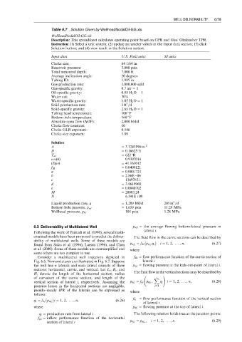
Table 6.7 Solution Given by WellheadNodalOil-GG.xls
WellheadNodalOil-GG.xls
Description: This spreadsheet calculates operating point based on CPR and Guo–Ghalambor TPR.
Instruction: (1) Select a unit system; (2) update parameter values in the Input data section; (3) click
Solution button; and (4) view result in the Solution section.
Input data U.S. Field units SI units
Choke size: 64 1/64 in.
Reservoir pressure: 3,000 psia
Total measured depth: 7,000 ft
Average inclination angle: 20 degrees
Tubing ID: 1.995 in.
Gas production rate: 1,000,000 scfd
Gas-specific gravity: 0.7 air ¼ 1
Oil-specific gravity: 0.85 H 2 O ¼ 1
Water cut: 30%
Water-specific gravity: 1.05 H 2 O ¼ 1
3
Solid production rate: 1 ft =d
Solid-specific gravity: 2.65 H 2 O ¼ 1
Tubing head temperature: 100 8F
Bottom-hole temperature: 160 8F
Absolute open flow (AOF): 2,000 bbl/d
Choke flow constant: 10
Choke GLR exponent: 0.546
Choke-size exponent: 1.89
Solution
A ¼ 3:1243196 in: 2
D ¼ 0.16625 ft
T av ¼ 622 8R
cos(u) ¼ 0.9397014
(Drv) ¼ 41.163012
f M ¼ 0.0409121
a ¼ 0.0001724
b ¼ 2.86E 06
c ¼ 1349785.1
d ¼ 3.8619968
e ¼ 0.0040702
M ¼ 20003.24
N ¼ 6.591Eþ09
3
Liquid production rate, q ¼ 1,289 bbl/d 205 m =d
Bottom hole pressure, p wf ¼ 1,659 psia 11.29 MPa
Wellhead pressure, p hf ¼ 188 psia 1.28 MPa

6.3 Deliverability of Multilateral Well p wf i ¼ the average flowing bottom-lateral pressure in
lateral i.
Following the work of Pernadi et al. (1996), several math-
ematical models have been proposed to predict the deliver- The fluid flow in the curvic sections can be described by
ability of multilateral wells. Some of these models are
found from Salas et al. (1996), Larsen (1996), and Chen p wf i ¼ f Ri p kf i ,q i i ¼ 1, 2, .. . , n, (6:27)
et al. (2000). Some of these models are oversimplified and where
some others are too complex to use.
Consider a multilateral well trajectory depicted in f Ri ¼ flow performance function of the curvic section of
Fig. 6.6. Nomenclatures are illustrated in Fig. 6.7. Suppose lateral i
the well has n laterals and each lateral consists of three p kf i ¼ flowing pressure at the kick-out-point of lateral i.
sections: horizontal, curvic, and vertical. Let L i , R i , and
H i denote the length of the horizontal section, radius The fluid flow in the vertical sections may be described by
!
of curvature of the curvic section, and length of the X
i
vertical section of lateral i, respectively. Assuming the p kf i ¼ f hi p hf i , q j i ¼ 1, 2, ... , n, (6:28)
pressure losses in the horizontal sections are negligible, j¼1
pseudo–steady IPR of the laterals can be expressed as where
follows:
f hi ¼ flow performance function of the vertical section
q i ¼ f L i p wf i i ¼ 1, 2, .. . , n, (6:26)
of lateral i
where p hf i ¼ flowing pressure at the top of lateral i.
q i ¼ production rate from lateral i The following relation holds true at the junction points:
f Li ¼ inflow performance function of the horizontal
i ¼ 1, 2, .. . , n (6:29)
section of lateral i p kf i ¼ p hf i 1