Page 83 - Petroleum Production Engineering, A Computer-Assisted Approach

Guo, Boyun / Computer Assited Petroleum Production Engg 0750682701_chap06 Final Proof page 75 3.1.2007 8:40pm Compositor Name: SJoearun

WELL DELIVERABILITY 6/75
7,000

6,000
Bottom Hole Pressure (psia) 4,000 IPR
5,000

TPR
3,000

2,000

1,000

0
0 1,000 2,000 3,000 4,000 5,000
Liquid Production Rate (bbl/d)
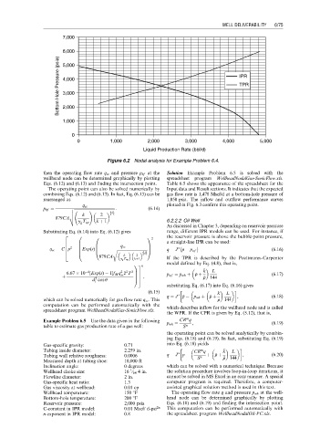
Figure 6.2 Nodal analysis for Example Problem 6.4.

then the operating flow rate q sc and pressure p hf at the Solution Example Problem 6.5 is solved with the
wellhead node can be determined graphically by plotting spreadsheet program WellheadNodalGas-SonicFlow.xls.
Eqs. (6.12) and (6.13) and finding the intersection point. Table 6.5 shows the appearance of the spreadsheet for the
The operating point can also be solved numerically by Input data and Result sections. It indicates that the expected
combining Eqs. (6.12) and (6.13). In fact, Eq. (6.13) can be gas flow rate is 1,478 Mscf/d at a bottom-hole pressure of
rearranged as 1,050 psia. The inflow and outflow performance curves
plotted in Fig. 6.3 confirm this operating point.
q sc
p hf ¼ v ffiffiffiffiffiffiffiffiffiffiffiffiffiffiffiffiffiffiffiffiffiffiffiffiffiffiffiffiffiffiffiffiffiffiffiffiffiffiffiffiffiffi : (6:14)
!
u
u k 2 kþ1
k 1
879CA t
g g T up k þ 1 6.2.2.2 Oil Well
As discussed in Chapter 3, depending on reservoir pressure
Substituting Eq. (6.14) into Eq. (6.12) gives range, different IPR models can be used. For instance, if
2 0 0 1 2 the reservoir pressure is above the bubble-point pressure,
6 B B C a straight-line IPR can be used:

6
B
q sc
2

p
6
q sc ¼ C p B Exp(s) B r ffiffiffiffiffiffiffiffiffiffiffiffiffiffiffiffiffiffiffiffiffiffiffiffiffiffiffiffiffiffiffi C q ¼ J p p wf (6:16)
p
@
4 @ kþ1A
879CA k 2 k 1
g g T up kþ1 If the TPR is described by the Poettmann–Carpenter
model defined by Eq. (4.8), that is,
13 n

2
6:67 10 [Exp(s) 1]f M q z T C7 p wf ¼ p wh þ r þ k k L (6:17)
4
2
2
z
T
r
þ sc C7 , r r 144
5
d cos u A5
i
substituting Eq. (6.17) into Eq. (6.16) gives

(6:15) k k L

q ¼ J p p p wh þ r þ , (6:18)
r
which can be solved numerically for gas flow rate q sc . This r r 144
computation can be performed automatically with the
spreadsheet program WellheadNodalGas-SonicFlow.xls. which describes inflow for the wellhead node and is called
the WPR. If the CPR is given by Eq. (5.12), that is,
m
Example Problem 6.5 Use the data given in the following p wh ¼ CR q , (6:19)
table to estimate gas production rate of a gas well: S n
the operating point can be solved analytically by combin-
ing Eqs. (6.18) and (6.19). In fact, substituting Eq. (6.19)
Gas-specific gravity: 0.71 into Eq. (6.18) yields
Tubing inside diameter: 2.259 in. CR q k k L
m
r

Tubing wall relative roughness: 0.0006 q ¼ J p p S n þ r þ r r 144 , (6:20)
Measured depth at tubing shoe: 10,000 ft
Inclination angle: 0 degrees which can be solved with a numerical technique. Because
1
Wellhead choke size: 16 ⁄ 64 4 in. the solution procedure involves loop-in-loop iterations, it
Flowline diameter: 2 in. cannot be solved in MS Excel in an easy manner. A special
Gas-specific heat ratio: 1.3 computer program is required. Therefore, a computer-
Gas viscosity at wellhead: 0.01 cp assisted graphical solution method is used in this text.
Wellhead temperature: 150 8F The operating flow rate q and pressure p wh at the well-
Bottom-hole temperature: 200 8F head node can be determined graphically by plotting
Reservoir pressure: 2,000 psia Eqs. (6.18) and (6.19) and finding the intersection point.
C-constant in IPR model: 0.01 Mscf/ d-psi 2n This computation can be performed automatically with
n-exponent in IPR model: 0.8 the spreadsheet program WellheadNodalOil-PC.xls.