Page 81 - Petroleum Production Engineering, A Computer-Assisted Approach

Guo, Boyun / Computer Assited Petroleum Production Engg 0750682701_chap06 Final Proof page 73 3.1.2007 8:40pm Compositor Name: SJoearun

WELL DELIVERABILITY 6/73
1 2bM
144b( p wf p hf ) þ Water-specific gravity: 1.05 H 2 O ¼ 1
2 Solid production rate: 1 ft =d
3
b Solid-specific gravity: 2.65 H 2 O ¼ 1
(144p wf þ M) þ N M þ N bM 2
2
ln c p ffiffiffiffiffi Tubing head temperature: 100 8F
2
(144p hf þ M) þ N N Bottom-hole temperature: 160 8F
144p wf þ M 144p hf þ M Tubing head pressure: 300 psia
tan 1 p ffiffiffiffiffi tan 1 p ffiffiffiffiffi Absolute open flow (AOF): 2,000 bbl/d
N N
2
¼ a( cos u þ d e)L, (6:10)
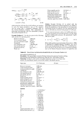
Solution Example Problem 6.3 is solved with the
substituting Eq. (6.9) into Eq. (6.10) will give an equation spreadsheet program BottomHoleNodalOil-GG.xls. Table 6.3
to solve for liquid production rate q. The equation shows the appearance of the spreadsheet for the Input data
can be solved with a numerical technique such as and Result sections. It indicates that the expected oil flow
the Newton–Raphson iteration. This computation is rate is 1,268 stb/d at a bottom-hole pressure of 1,688 psia.
performed automatically with the spreadsheet program
BottomHoleNodalOil-GG.xls. If the reservoir pressure is above the bubble-point pres-
sure, but the flowing bottom-hole pressure is in the range
of below bubble-point pressure, the generalized Vogel’s
Example Problem 6.3 For the data given in the following
table, predict the operating point: IPR can be used: #
"
Reservoir pressure: 3,000 psia p wf p wf 2
Total measured depth: 7,000 ft q ¼ q b þ q v 1 0:2 0:8 (6:11)
p b p b
Average inclination angle: 20 degree
Tubing ID: 1.995 in. Iftheoutflowperformancerelationshipofthenode(i.e.,TPR)
Gas production rate: 1,000,000 scfd is described by Hagedorn-Brown correlation, Eq. (4.27)
Gas-specific gravity: 0.7 air ¼ 1 can be used for generating the TPR curve. Combining Eqs.
Oil-specific gravity: 0.85 H 2 O ¼ 1 (6.11) and (4.27) can be solved with a numerical technique
Water cut: 30 % such as the Newton–Raphson iteration for liquid flow rate
Table 6.3 Result Given by BottomHoleNodalOil-GG.xls for Example Problem 6.2
BottomHoleNodalOil-GG.xls
Description: This spreadsheet calculates flowing bottom-hole pressure based on tubing
head pressure and tubing flow performance using the Guo–Ghalambor method.
Instruction: (1) Select a unit system; (2) update parameter values in the Input data
section; (3) click Result button; and (4) view result in the Result section.
Input data U.S. Field units SI units
Reservoir pressure: 3,000 psia
Total measured depth: 7,000 ft
Average inclination angle: 20 degrees
Tubing ID: 1.995 in.
Gas production rate: 1,000,000 scfd
Gas-specific gravity: 0.7 air ¼ 1
Oil-specific gravity: 0.85 H 2 O ¼ 1
Water cut: 30%
Water-specific gravity: 1.05 H 2 O ¼ 1
3
Solid production rate: 1 ft =d
Solid-specific gravity: 2.65 H 2 O ¼ 1
Tubing head temperature: 100 8F
Bottom-hole temperature: 160 8F
Tubing head pressure: 300 psia
Absolute open flow (AOF): 2000 bbl/d
Solution
A ¼ 3:1243196 in: 2
D ¼ 0.16625 ft
T av ¼ 622 8R
cos (u) ¼ 0.9397014
(Drv) ¼ 40.576594
f M ¼ 0.0424064
a ¼ 0.0001699
b ¼ 2.814E-06
c ¼ 1,349,785.1
d ¼ 3.7998147
e ¼ 0.0042189
M ¼ 20,395.996
N ¼ 6.829Eþ09
Liquid production rate, q ¼ 1,268 bbl/d
Bottom hole pressure, p wf ¼ 1,688 psia