Page 390 - A First Course In Stochastic Models

MULTI-SERVER QUEUES WITH POISSON INPUT 385

e
e
S , . . . , S are independent random variables that have the equilibrium excess dis-
1 k
tribution function
1 t
B e (t) = {1 − B(x)}dx, t ≥ 0,
E(S) 0
as probability distribution function.
(b) If at a service completion epoch, k customers are left behind in the system
with k ≥ c, then the time until the next service completion is distributed as S/c,
where S denotes the original service time of a customer.
This approximation assumption can be motivated as follows. First, if not all
c servers are busy, the M/G/c queueing system may be treated as an M/G/∞
queueing system in which a free server is immediately provided to each arriving
customer. For the M/G/∞ queue in statistical equilibrium it was shown by Tak´ acs
(1962) that the remaining service time of any busy server is distributed as the
residual life in a renewal process with the service times as the interoccurrence
times. The same is true for the M/G/1 queue; see formula (9.2.32). The equilibrium
excess distribution of the service time is given by B e (t); see Theorem 8.2.5. Second,
if all of the c servers are busy, then the M/G/c queue may be approximated by
an M/G/1 queue in which the single server works c times as fast as each of the c
servers in the original multi-server system. It is pointed out that the approximation
assumption holds exactly for both the case of the c = 1 server and the case of
exponentially distributed service times.

Approximations to the state probabilities
Under the approximation assumption the recursion scheme derived in Section 9.2.1
for the M/G/1 queue can be extended to the M/G/c queue to yield approximations
app
p to the state probabilities p j . These approximations are given in the next
j
theorem, whose lengthy proof may be skipped at first reading. The approximation
to the state probabilities implies an approximation to the waiting-time probabilities.
The latter approximation is discussed in Exercise 9.11.
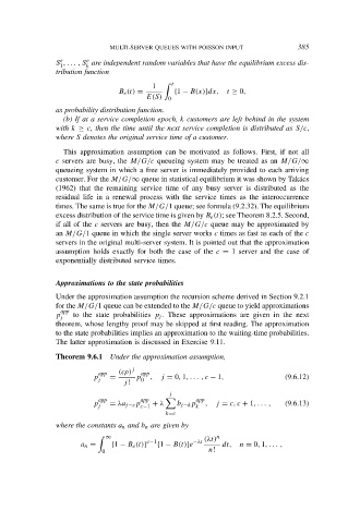
Theorem 9.6.1 Under the approximation assumption,

app (cρ) j app
p = p , j = 0, 1, . . . , c − 1, (9.6.12)
j 0
j!
j
app app app
p = λa j−c p + λ b j−k p , j = c, c + 1, . . . , (9.6.13)
j c−1 k
k=c
where the constants a n and b n are given by
n
∞ (λt)
c−1 −λt
a n = {1 − B e (t)} {1 − B(t)}e dt, n = 0, 1, . . . ,
0 n!