Page 391 - A First Course In Stochastic Models

386 ALGORITHMIC ANALYSIS OF QUEUEING MODELS

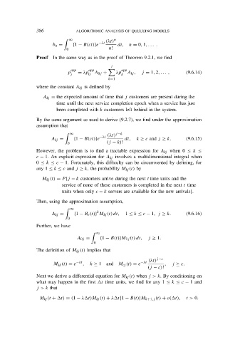
n
∞ (λt)
b n = {1 − B(ct)}e −λt dt, n = 0, 1, . . . .
0 n!
Proof In the same way as in the proof of Theorem 9.2.1, we find
j
app app app
p = λp A 0j + λp A kj , j = 1, 2, . . . , (9.6.14)
j 0 k
k=1
where the constant A kj is defined by

A kj = the expected amount of time that j customers are present during the
time until the next service completion epoch when a service has just
been completed with k customers left behind in the system.

By the same argument as used to derive (9.2.7), we find under the approximation
assumption that

∞ (λt)
j−k
A kj = {1 − B(ct)}e −λt dt, k ≥ c and j ≥ k. (9.6.15)
0 (j − k)!
However, the problem is to find a tractable expression for A kj when 0 ≤ k ≤
c − 1. An explicit expression for A kj involves a multidimensional integral when
0 ≤ k ≤ c − 1. Fortunately, this difficulty can be circumvented by defining, for
any 1 ≤ k ≤ c and j ≥ k, the probability M kj (t) by
M kj (t) = P {j − k customers arrive during the next t time units and the
service of none of these customers is completed in the next t time
units when only c − k servers are available for the new arrivals}.
Then, using the approximation assumption,

∞

k
A kj = {1 − B e (t)} M kj (t) dt, 1 ≤ k ≤ c − 1, j ≥ k. (9.6.16)
0
Further, we have

∞
A 0j = {1 − B(t)}M 1j (t) dt, j ≥ 1.
0
The definition of M kj (t) implies that
(λt) j−c
−λt
−λt
M kk (t) = e , k ≥ 1 and M cj (t) = e , j ≥ c.
(j − c)!
Next we derive a differential equation for M kj (t) when j > k. By conditioning on
what may happen in the first t time units, we find for any 1 ≤ k ≤ c − 1 and
j > k that

M kj (t + t) = (1 − λ t)M kj (t) + λ t{1 − B(t)}M k+1,j (t) + o( t), t > 0.