Page 93 - A Guide to MATLAB for Beginners and Experienced Users

74 Chapter 5: MATLAB Graphics

4
3
2
1

0
-1
-2
-3
-4
2
1 2
1
0
0
-1
-1
-2 -2
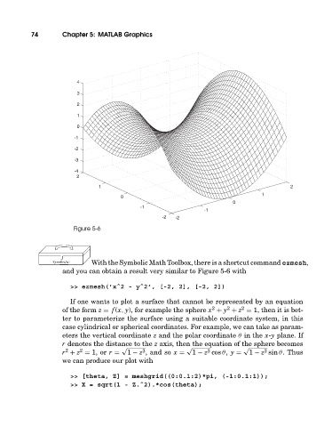
Figure 5-6

With the Symbolic Math Toolbox, there is a shortcut command ezmesh,
and you can obtain a result very similar to Figure 5-6 with

>> ezmesh(’xˆ2 - yˆ2’, [-2, 2], [-2, 2])

If one wants to plot a surface that cannot be represented by an equation
2
2
2
of the form z = f (x, y), for example the sphere x + y + z = 1, then it is bet-
ter to parameterize the surface using a suitable coordinate system, in this
case cylindrical or spherical coordinates. For example, we can take as param-
eters the vertical coordinate z and the polar coordinate θ in the x-y plane. If
r denotes the distance to the z axis, then the equation of the sphere becomes
√ √ √
2 2 2 2 2
r + z = 1, or r = 1 − z , and so x = 1 − z cos θ, y = 1 − z sin θ. Thus
we can produce our plot with
>> [theta, Z] = meshgrid((0:0.1:2)*pi, (-1:0.1:1));
>> X = sqrt(1 - Z.ˆ2).*cos(theta);