Page 120 - Acquisition and Processing of Marine Seismic Data

2.4 SPECIFIC ACQUISITION TECHNIQUES 111

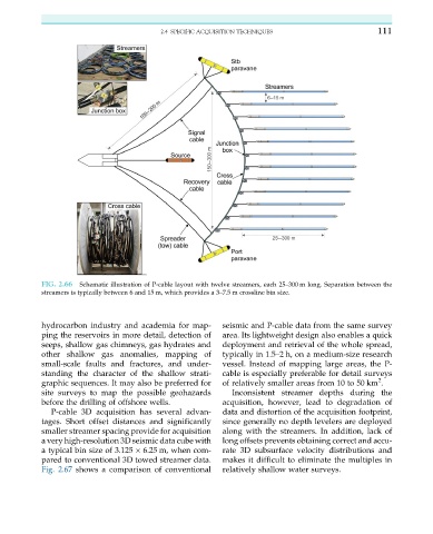
FIG. 2.66 Schematic illustration of P-cable layout with twelve streamers, each 25–300 m long. Separation between the
streamers is typically between 6 and 15 m, which provides a 3–7.5 m crossline bin size.

hydrocarbon industry and academia for map- seismic and P-cable data from the same survey
ping the reservoirs in more detail, detection of area. Its lightweight design also enables a quick
seeps, shallow gas chimneys, gas hydrates and deployment and retrieval of the whole spread,
other shallow gas anomalies, mapping of typically in 1.5–2 h, on a medium-size research
small-scale faults and fractures, and under- vessel. Instead of mapping large areas, the P-
standing the character of the shallow strati- cable is especially preferable for detail surveys
2
graphic sequences. It may also be preferred for of relatively smaller areas from 10 to 50 km .
site surveys to map the possible geohazards Inconsistent streamer depths during the
before the drilling of offshore wells. acquisition, however, lead to degradation of
P-cable 3D acquisition has several advan- data and distortion of the acquisition footprint,
tages. Short offset distances and significantly since generally no depth levelers are deployed
smaller streamer spacing provide for acquisition along with the streamers. In addition, lack of
a very high-resolution 3D seismic data cube with long offsets prevents obtaining correct and accu-
a typical bin size of 3.125 6.25 m, when com- rate 3D subsurface velocity distributions and
pared to conventional 3D towed streamer data. makes it difficult to eliminate the multiples in
Fig. 2.67 shows a comparison of conventional relatively shallow water surveys.