Page 224 - Acquisition and Processing of Marine Seismic Data

4.3 CONVOLUTION 215

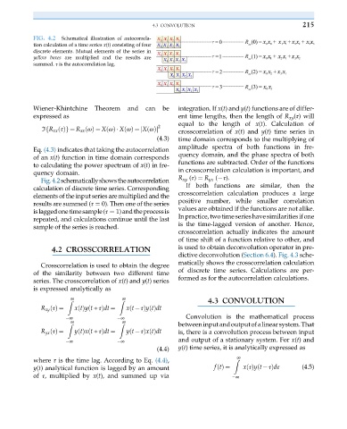
FIG. 4.2 Schematical illustration of autocorrela-
tion calculation of a time series x(t)consisting offour
discrete elements. Mutual elements of the series in
yellow boxes are multiplied and the results are
summed. τ is the autocorrelation lag.

Wiener-Khintchine Theorem and can be integration. If x(t) and y(t) functions are of differ-
expressed as ent time lengths, then the length of R xy (τ) will
equal to the length of x(t). Calculation of
2
ℑ R xx τðÞg ¼ R xx ωðÞ ¼ X ωðÞ X ωðÞ ¼ X ωðÞj
f
j
crosscorrelation of x(t) and y(t) time series in
(4.3) time domain corresponds to the multiplying of
amplitude spectra of both functions in fre-
Eq. (4.3) indicates that taking the autocorrelation
quency domain, and the phase spectra of both
of an x(t) function in time domain corresponds
functions are subtracted. Order of the functions
to calculating the power spectrum of x(t) in fre-
in crosscorrelation calculation is important, and
quency domain.
R xy (τ) ¼ R yx ( τ).
Fig.4.2schematicallyshowstheautocorrelation
calculation of discrete time series. Corresponding If both functions are similar, then the
elements of the input series are multiplied and the crosscorrelation calculation produces a large
results are summed (τ ¼ 0). Then one of the series positive number, while smaller correlation
islaggedonetimesample(τ ¼ 1)andtheprocessis values are obtained if the functions are not alike.
repeated, and calculations continue until the last Inpractice,twotimeserieshavesimilaritiesifone
is the time-lagged version of another. Hence,
sample of the series is reached.
crosscorrelation actually indicates the amount
of time shift of a function relative to other, and
4.2 CROSSCORRELATION is used to obtain deconvolution operator in pre-
dictive deconvolution (Section 6.4). Fig. 4.3 sche-
matically shows the crosscorrelation calculation
Crosscorrelation is used to obtain the degree
of the similarity between two different time of discrete time series. Calculations are per-
series. The crosscorrelation of x(t) and y(t) series formed as for the autocorrelation calculations.
is expressed analytically as
Z ∞ Z ∞ 4.3 CONVOLUTION

ð
ð
R xy τðÞ ¼ xtðÞyt + τÞdt ¼ xt τÞytðÞdt
∞ ∞ Convolution is the mathematical process
Z ∞ Z ∞ betweeninputandoutputofalinearsystem.That
ð
R yx τðÞ ¼ ytðÞxt + τÞdt ¼ yt τÞxtðÞdt is, there is a convolution process between input
ð
∞ ∞ and output of a stationary system. For x(t) and
(4.4) y(t) time series, it is analytically expressed as
Z ∞
where τ is the time lag. According to Eq. (4.4),
y(t) analytical function is lagged by an amount ftðÞ ¼ x τðÞyt τÞdτ (4.5)
ð
of τ, multiplied by x(t), and summed up via ∞