Page 225 - Acquisition and Processing of Marine Seismic Data

216 4. FUNDAMENTALS OF DATA PROCESSING

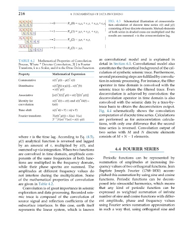
FIG. 4.3 Schematical illustration of crosscorrela-
tion calculation of discrete time series x(t) and y(t)
consisting of four discrete elements. Mutual elements
of both series in shaded areas are multiplied and the
results are summed. τ is the crosscorrelation lag.

as convolutional model and is explained in
TABLE 4.2 Mathematical Properties of Convolution
Process, Where * Denotes Convolution, ℑ{ } is Fourier detail in Section 6.1. Convolutional model also
Transform, k is a Scalar, and δ is the Dirac Delta Function constitutes the theoretical background of the cal-
culation of synthetic seismic trace. Furthermore,
several processing steps are fulfilled by convolu-
Property Mathematical Expression
∗ ∗
Commutative x(t) y(t)¼y(t) x(t) tion in seismic processing. For instance, the filter
∗ ∗
Distributive x(t) [f(t)+y(t)]¼x(t) f(t) operator in time domain is convolved with the
∗
+x(t) y(t) seismic trace to obtain the filtered trace. Even
∗ ∗ ∗ ∗ deconvolution is achieved by convolution: the
Associative [x(t) f(t)] y(t)¼x(t) [f(t) y(t)]
deconvolution operator in time domain is also
∗
∗
Identity for x(t) δ(t)¼x(t) and x(t) kδ(t)¼ convolved with the seismic data by a trace-by-
convolution kx(t)
trace basis to obtain the deconvolution output.
∗
Time shift x(t) δ(t+T)¼x(t+T) Fig. 4.4 schematically shows the convolution
∗
Fourier transform ℑ{x(t) y(t)}¼X(ω) Y(ω) computation of discrete time series. Calculations
∗
1
ℑ {X(ω) Y(ω)}¼x(t) y(t) are performed as for autocorrelation calcula-
tions, with only one difference that the second
time series is reversed. Convolution output of
two series with M and N discrete elements
where τ is the time lag. According to Eq. (4.5), consists of M + N 1 elements.
y(t) analytical function is reversed and lagged
by an amount of τ, multiplied by x(t), and
summed up via integration. When two functions 4.4 FOURIER SERIES
are convolved in time domain, amplitude com-
ponents of the same frequencies of both func- Periodic functions can be represented by
tions are multiplied in the frequency domain, summation of amplitudes at increasing fre-
while their phase spectra are summed. The quency values of two orthogonal functions. Jean
amplitudes at different frequency values do Baptiste Joseph Fourier (1768–1830) accom-
not interfere during the multiplication. Some plished this summation by using sine and cosine
of the mathematical properties of convolution functions. Periodic functions can be decom-
are given in Table 4.2. posed into sinusoidal harmonics, which means
Convolution is of great importance in seismic that any kind of periodic function can be
exploration and data processing. Recorded seis- expressed as weighted summation of infinite
mic trace is composed of the convolution of number of sine and cosine functions with differ-
source signal and reflection coefficients of the ent amplitude, phase and frequency values
subsurface interfaces. In this case, earth itself using Fourier series summation approximation
represents the linear system, which is known in such a way that, using orthogonal sine and