Page 226 - Acquisition and Processing of Marine Seismic Data

4.4 FOURIER SERIES 217

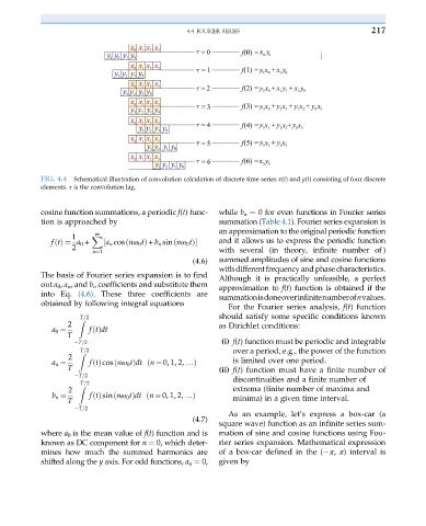
FIG. 4.4 Schematical illustration of convolution calculation of discrete time series x(t) and y(t) consisting of four discrete
elements. τ is the convolution lag.

cosine function summations, a periodic f(t) func- while b n ¼ 0 for even functions in Fourier series
tion is approached by summation (Table 4.1). Fourier series expansion is
∞ an approximation to the original periodic function
1 X
ftðÞ ¼ a 0 + ½ a n cos nω 0 tÞ + b n sin nω 0 tފ and it allows us to express the periodic function
ð
ð
2
n¼1 with several (in theory, infinite number of )
(4.6) summed amplitudes of sine and cosine functions
with different frequency and phase characteristics.
The basis of Fourier series expansion is to find Although it is practically unfeasible, a perfect
out a 0 , a n , and b n coefficients and substitute them approximation to f(t)functionisobtainedifthe
into Eq. (4.6). These three coefficients are summationisdoneoverinfinitenumberofnvalues.
obtained by following integral equations
For the Fourier series analysis, f(t) function
T=2 should satisfy some specific conditions known
2 Z as Dirichlet conditions:
a 0 ¼ ftðÞdt
T
T=2 (i) f(t) function must be periodic and integrable
T=2 over a period, e.g., the power of the function
2 Z
a n ¼ ftðÞcos nω 0 tÞdt n ¼ 0, 1, 2, …Þ is limited over one period.
ð
ð
T (ii) f(t) function must have a finite number of
T=2 discontinuities and a finite number of
T=2
2 Z extrema (finite number of maxima and
b n ¼ ftðÞsin nω 0 tÞdt n ¼ 0, 1, 2, …Þ minima) in a given time interval.
ð
ð
T
T=2
As an example, let’s express a box-car (a
(4.7)
square wave) function as an infinite series sum-
where a 0 is the mean value of f(t) function and is mation of sine and cosine functions using Fou-
known as DC component for n ¼ 0, which deter- rier series expansion. Mathematical expression
mines how much the summed harmonics are of a box-car defined in the ( π, π) interval is
shifted along the y axis. For odd functions, a n ¼ 0, given by