Page 174 - Adaptive Identification and Control of Uncertain Systems with Nonsmooth Dynamics

170 Adaptive Identification and Control of Uncertain Systems with Non-smooth Dynamics

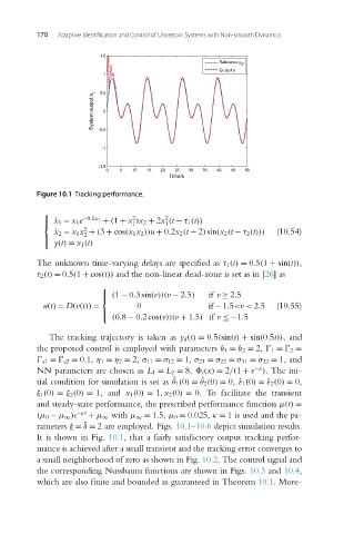
Figure 10.1 Tracking performance.

⎧
2
2
⎪ ˙ x 1 = x 1e −0.5x 1 + (1 + x )x 2 + 2x (t − τ 1 (t))
⎨ 1 1
2
˙ x 2 = x 1x + (3 + cos(x 1x 2 ))u + 0.2x 2 (t − 2)sin(x 2 (t − τ 2 (t))) (10.54)
2
y(t) = x 1 (t)
⎪
⎩
The unknown time-varying delays are specified as τ 1 (t) = 0.5(1 + sin(t)),
τ 2 (t) = 0.5(1 + cos(t)) and the non-linear dead-zone is set as in [26]as
⎧
⎪ (1 − 0.3sin(v))(v − 2.5) if v ≥ 2.5
⎨
u(t) = D(v(t)) = 0 if − 1.5<v < 2.5 (10.55)
⎪
⎩ (0.8 − 0.2cos(v))(v + 1.5) if v ≤−1.5
The tracking trajectory is taken as y d (t) = 0.5(sin(t) + sin(0.5t)),and
the proposed control is employed with parameters k 1 = k 2 = 2, 1 = 2 =
a1 = a2 = 0.1, η 1 = η 2 = 2, σ 11 = σ 12 = 1, σ 21 = σ 22 = σ 31 = σ 32 = 1, and
−x
NN parameters are chosen as L 1 = L 2 = 8, i (x) = 2/(1 + e ). The ini-
tial condition for simulation is set as θ 1 (0) = θ 2 (0) = 0, ˆε 1 (0) =ˆε 2 (0) = 0,
ˆ
ˆ
ξ 1 (0) = ξ 2 (0) = 1, and x 1 (0) = 1,x 2 (0) = 0. To facilitate the transient
and steady-state performance, the prescribed performance function μ(t) =
(μ 0 − μ ∞ )e −κt + μ ∞ with μ ∞ = 1.5, μ 0 = 0.025, κ = 1is used and the pa-
¯
rameters δ = δ = 2 are employed. Figs. 10.1–10.6 depict simulation results.
It is shown in Fig. 10.1, that a fairly satisfactory output tracking perfor-
mance is achieved after a small transient and the tracking error converges to
a small neighborhood of zero as shown in Fig. 10.2. The control signal and
the corresponding Nussbaum functions are shown in Figs. 10.3 and 10.4,
which are also finite and bounded as guaranteed in Theorem 10.1. More-