Page 351 - Advanced engineering mathematics

10.6 Phase Portraits 331

y
y
L 1
L 2
L
E 1 P 0 1
E 2 T 3
P 0
x
L 2
P 0 T 1
T 2
x

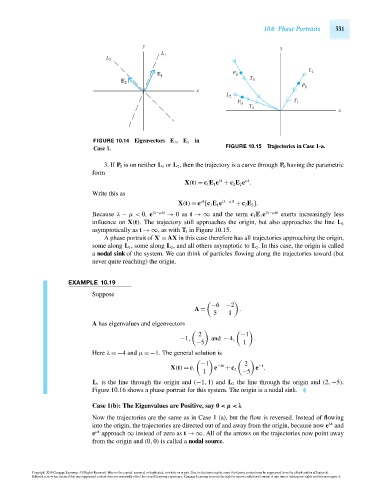
FIGURE 10.14 Eigenvectors E 1 , E 2 in
Case 1. FIGURE 10.15 Trajectories in Case 1-a.

3. If P 0 is on neither L 1 or L 2 , then the trajectory is a curve through P 0 having the parametric
form
λt
μt
X(t) = c 1 E 1 e + c 2 E 2 e .
Write this as
μt
X(t) = e [c 1 E 1 e (λ−μ)t + c 2 E 2 ].
Because λ − μ< 0, e (λ−μ)t → 0as t →∞ and the term c 1 E 1 e (λ−μ)t exerts increasingly less
influence on X(t). The trajectory still approaches the origin, but also approaches the line L 2
asymptotically as t →∞, as with T 3 in Figure 10.15.
A phase portrait of X =AX in this case therefore has all trajectories approaching the origin,

some along L 1 , some along L 2 , and all others asymptotic to L 2 . In this case, the origin is called
a nodal sink of the system. We can think of particles flowing along the trajectories toward (but
never quite reaching) the origin.

EXAMPLE 10.19
Suppose

−6 −2
A = .
5 1
A has eigenvalues and eigenvectors

2 −1
−1, and − 4, .
−5 1
Here λ =−4 and μ =−1. The general solution is

−1 −4t 2 −t
X(t) = c 1 e + c 2 e .
1 −5
L 1 is the line through the origin and (−1,1) and L 2 the line through the origin and (2,−5).
Figure 10.16 shows a phase portrait for this system. The origin is a nodal sink.

Case 1(b): The Eigenvalues are Positive, say 0 <μ<λ
Now the trajectories are the same as in Case 1 (a), but the flow is reversed. Instead of flowing
λt
into the origin, the trajectories are directed out of and away from the origin, because now e and
μt
e approach ∞ instead of zero as t →∞. All of the arrows on the trajectories now point away
from the origin and (0,0) is called a nodal source.

Copyright 2010 Cengage Learning. All Rights Reserved. May not be copied, scanned, or duplicated, in whole or in part. Due to electronic rights, some third party content may be suppressed from the eBook and/or eChapter(s).
Editorial review has deemed that any suppressed content does not materially affect the overall learning experience. Cengage Learning reserves the right to remove additional content at any time if subsequent rights restrictions require it.

October 14, 2010 20:32 THM/NEIL Page-331 27410_10_ch10_p295-342