Page 354 - Advanced engineering mathematics

334 CHAPTER 10 Systems of Linear Differential Equations

y
10
y

5

x
–10 –5 0 5 10
x
–5

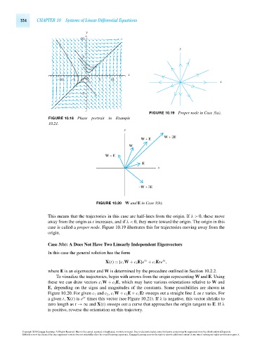
FIGURE 10.19 Proper node in Case 3(a).
FIGURE 10.18 Phase portrait in Example
10.21.
y
W + 2E
W + E
W
W − E
E
x

−W + 2E

FIGURE 10.20 W and E in Case 3(b).

This means that the trajectories in this case are half-lines from the origin. If λ> 0, these move
away from the origin as t increases, and if λ< 0, they move toward the origin. The origin in this
case is called a proper node. Figure 10.19 illustrates this for trajectories moving away from the
origin.

Case 3(b): A Does Not Have Two Linearly Independent Eigenvectors

In this case the general solution has the form
λt
λt
X(t) =[c 1 W + c 2 E]e + c 1 Ete ,
where E is an eigenvector and W is determined by the procedure outlined in Section 10.2.2.
To visualize the trajectories, begin with arrows from the origin representing W and E.Using
these we can draw vectors c 1 W + c 2 E, which may have various orientations relative to W and
E, depending on the signs and magnitudes of the constants. Some possibilities are shown in
Figure 10.20. For given c 1 and c 2 , c 1 W + c 2 E + c 1 Et sweeps out a straight line L as t varies. For
λt
agiven t, X(t) is e times this vector (see Figure 10.21). If λ is negative, this vector shrinks to
zero length as t →∞ and X(t) sweeps out a curve that approaches the origin tangent to E.If λ
is positive, reverse the orientation on this trajectory.

Copyright 2010 Cengage Learning. All Rights Reserved. May not be copied, scanned, or duplicated, in whole or in part. Due to electronic rights, some third party content may be suppressed from the eBook and/or eChapter(s).
Editorial review has deemed that any suppressed content does not materially affect the overall learning experience. Cengage Learning reserves the right to remove additional content at any time if subsequent rights restrictions require it.

October 14, 2010 20:32 THM/NEIL Page-334 27410_10_ch10_p295-342