Page 355 - Advanced engineering mathematics

10.6 Phase Portraits 335

y

L
c W + c E + c Et
1
1
2
X(t)
W
E
x

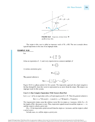
FIGURE 10.21 Trajectory formed from W
and E in Case 3(b).

The origin in this case is called an improper node of X = AX. The next example shows

typical trajectories in the case of an improper node.

EXAMPLE 10.22
Let

−10 6
A = .
−6 2
A has an eigenvalue of −4, and every eigenvector is a nonzero multiple of

1
E = .
1
A routine calculation gives
1

W = .
7/6
The general solution is

t + 1 −4t 1 −4t
X(t) = c 1 e + c 2 e .
t + 7/6 1
Figure 10.22 is a phase portrait for this system. The trajectories approach the origin tangent to
the line through E, when this vector is represented as an arrow from the origin. The origin is an
improper node for this system.

Case 4: A Has Complex Eigenvalues With Nonzero Real Part
Let λ = α + iβ be an eigenvalue with α = 0 and eigenvector U + iV. Then the general solution is
αt
αt
X(t) = c 1 e [Ucos(βt) − vsin(βt)]+ c 2 e [Usin(βt) + Vsin(βt)].
The trigonometric terms cause the solution vector X(t) to rotate as t increases, while if α< 0,
the length of X(t) decreases to zero. Thus, trajectories spiral inward toward the origin as t →∞
and the origin is called a spiral sink.
If α>0, the trajectories spiral outward from the origin as t increases, and the origin is called
a spiral source.
In both cases, we call the origin a spiral point.

Copyright 2010 Cengage Learning. All Rights Reserved. May not be copied, scanned, or duplicated, in whole or in part. Due to electronic rights, some third party content may be suppressed from the eBook and/or eChapter(s).
Editorial review has deemed that any suppressed content does not materially affect the overall learning experience. Cengage Learning reserves the right to remove additional content at any time if subsequent rights restrictions require it.

October 14, 2010 20:32 THM/NEIL Page-335 27410_10_ch10_p295-342