Page 357 - Advanced engineering mathematics

10.6 Phase Portraits 337

Case 5: A Has Pure Imaginary Eigenvalues
Now trajectories have the form
X(t) = c 1 [Ucos(βt) − Vsin(βt)]+ c 2 [Usin(βt) + Vcos(βt)].
Without an exponential factor to increase or decrease the length of this vector, trajectories now
are closed curves about the origin, representing a periodic solution. Now the origin is called a
center of the system.
In general, closed trajectories of a system represent periodic solutions.

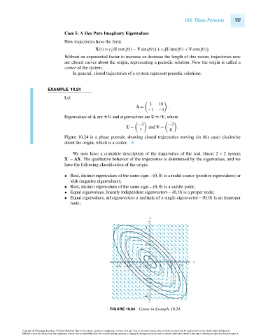
EXAMPLE 10.24

Let

3 18
A = .
−1 −3
Eigenvalues of A are ±3i and eigenvectors are U ± iV, where

−3 −3
U = and V = .
1 0
Figure 10.24 is a phase portrait, showing closed trajectories moving (in this case) clockwise
about the origin, which is a center.

We now have a complete description of the trajectories of the real, linear 2 × 2system
X = AX. The qualitative behavior of the trajectories is determined by the eigenvalues, and we

have the following classification of the origin:

• Real, distinct eigenvalues of the same sign—(0,0) is a nodal source (positive eigenvalues) or
sink (negative eigenvalues);
• Real, distinct eigenvalues of the same sign—(0,0) is a saddle point;
• Equal eigenvalues, linearly independent eigenvectors—(0,0) is a proper node;
• Equal eigenvalues, all eigenvectors a multiple of a single eigenvector—(0,0) is an improper
node;

y

4

2

x
–15 –10 –5 0 5 10 15

–2

–4

FIGURE 10.24 Center in Example 10.24.

Copyright 2010 Cengage Learning. All Rights Reserved. May not be copied, scanned, or duplicated, in whole or in part. Due to electronic rights, some third party content may be suppressed from the eBook and/or eChapter(s).
Editorial review has deemed that any suppressed content does not materially affect the overall learning experience. Cengage Learning reserves the right to remove additional content at any time if subsequent rights restrictions require it.

October 14, 2010 20:32 THM/NEIL Page-337 27410_10_ch10_p295-342