Page 13 - Advances in Biomechanics and Tissue Regeneration

1.3 PATIENT-SPECIFIC GEOMETRY 7

where A is a 3 3 constant matrix, B is a 3 1 constant vector, and c is a scalar, which defines the parameters of the
surface. Eq. (1.1) is fitted to the topographical data by means of a nonlinear regression analysis.
To extend the corneal surface, the quadric surface, Eq. (1.1) should properly approximate the periphery of the
patient’s topographical data. For this reason and before fitting Eq. (1.1), the central corneal part is removed using a
level-set algorithm based on the relative elevation of each corneal point with respect to the apex (for further details
see Ref. [12]).
When using an analytical surface such as Eq. (1.1) to extend the corneal surface, there will always be a jump at the
joint between the approximating surface and the point cloud surface (see Fig. 1.2B). This discontinuity in the normal of
the surface may lead to convergence problems or to nonrealistic stress distributions on the cornea during FE analysis.
Hence, a smoothing algorithm based on the continuity of the normal between the quadric surface and the point cloud
data is applied, as shown in Fig. 1.2B, producing local alterations in the patient’s topographic data near the border.
However, these alterations are very small (less than 3%) as outlined in the contour map of the error between the topo-
graphic point cloud data prior and after smoothing (Fig. 1.2C), where the depicted data corresponds to an extreme
post-LASIK patient.

1.3.2 Corneal Surface Finite Element Model
Once the corneal surface fitting is completed, it is introduced in the 3D model of the anterior half ocular globe,
which accounts for three different parts: the cornea, the limbus, and the sclera. Because only the cornea can be par-
tially measured by a topographer and neither the sclera nor thelimbuscan be measured withthisprocedure,average
parts are used instead. The sclera was assumed as a 25 mm in diameter sphere with a constant thickness of 1 mm,
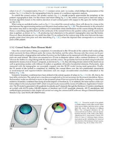
whereas the limbus is a ring linking both the sclera and the cornea. The geometry has been meshed using hexahedral
elements by means of an in-house C program, as shown in Fig. 1.3A, thus allowing precise control of the mesh size as
well as generating meshes with trilinear (8 nodes) or quadratic (20 nodes) hexahedral elements. Pachymetry data
measured with the topographer are accurately mapped onto the 3D FE model during mesh generation. Finally,
the FE model of the eyeball is completed by defining the corneal fibers over the two preferential orientations
(a nasal-temporal and superior-inferior directions) and one single circumferential orientation embedded in the
limbus (Fig. 1.3B).
Symmetry boundary conditions have been defined at the scleral equator (Π plane in Fig. 1.3A) [41, 42], that is, the
base of the semisclera. The optical nerve insertion was neglected as it is not necessary for the present simulation. Hence,
the boundary nodes are allowed to move on the symmetry plane Π but not normal to the plane, resulting in a much less
restrictive boundary condition than fixing all nodal degrees of freedom [6, 7]. In addition, the inner surface of the eye-
ball is subject to the actual patient’s IOP, which was previously measured by means of Goldmann Applanation Tonom-
etry. The FE model is generated with quadratic hexahedra and 5 elements through the thickness (11 nodes), resulting in
an eyeball with 62,276 nodes (186,828 degrees of freedom) and 13,425 quadratic elements. All FE simulations and
methodologies presented in this chapter are carried out using the commercial FE software Abaqus (Dassault Systemes
Simulia Corp.) and MATLAB (MathWorks).

FIG. 1.3 Numerical model of the eyeball.
(A) Finite element mesh of the eyeball: Sclera
(white region), limbus (dark blue region), cornea
(light blue region); (B) direction of collagen
fibers. Two orthogonal directions for the
cornea (red and green fibers), and one circum-
ferential direction of the limbus (blue fibers).
Adapted from M.Á. Ariza-Gracia, J. Zurita, D.P.
Piñero, B. Calvo, J.F. Rodríguez Matas, Automa-
tized patient-specific methodology for numerical
determination of biomechanical corneal response,
Ann. Biomed. Eng. 44 (5) (2016) 1753–1772.

I. BIOMECHANICS