Page 321 - Advances in Biomechanics and Tissue Regeneration

16.4 MATHEMATICAL FRAMEWORK 319

16.4.2 Physical Models for Fluxes and Sources
In order to close the partial differential equation system (PDEs) given by Eqs. (16.1), (16.4), we need to model the bio-
logical transport phenomena, that is, to make explicit the relations between the flux vector fields q i and q and other
0
i
physical variables that promote or inhibit cell migration (and/or substance diffusion) such as temperature (thermo-
taxis), electric potential (electrotaxis), substrate stiffness (durotaxis), strain (tensotaxis) (these latter two are usually
included under the term mechanotaxis), or chemical species concentration (chemotaxis) as well as cell concentrations
themselves (proper diffusion by random walk).
In addition to cell migration, growth, and differentiation of cellular phenotypes and consumption and production of
chemical species, the reaction terms can also be dependent on similar variables, so they have to be expressed in terms of
the same fields.

16.4.2.1 Source Terms in Cell Population Equations
First, the source terms in Eq. (16.1), which include proliferation F i and differentiation F ij , will be analyzed.

16.4.2.1.1 PROLIFERATION
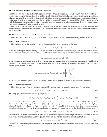
The proliferation of the ith phenotype can be expressed using an equation of the type:
F i ¼F i ðC 1 ,…,C n ,S 1 ,…,S m ,θ,p 1 ,…,p k Þ, i ¼ 1,…,n (16.7)

Here, θ is the temperature field and p 1 , …, p k are mechanical parameters characterizing the substrate (stiffness, anisot-
ropy if required, strain, etc.). An example of proliferation models is the exponential growth model where F i is written
as

F i ðC 1 ,…,C n ,S 1 ,…,S m ,θ,p 1 ,…,p k Þ¼ rðθÞ
with r the growth rate, depending only on the temperature, independent on the current concentration, and leading
therefore to an exponential growth of the number of cells per unit volume. Another possible model is the so-called
logistic growth model, where
n
0 1
X
C j
B C
j¼1
B C
B C
F i ðC 1 ,…,C n ,S 1 ,…,S m ,θ,p 1 ,…,p k Þ¼ r max ðθÞ 1
B C
@ C sat A
with r max the maximum growth rate, depending also on the temperature, and C sat the saturation parameter.
16.4.2.1.2 DIFFERENTIATION
The differentiation of the ith phenotype to the jth phenotype can be modeled using a similar equation:
F ij ¼F ij ðC 1 ,…,C n ,S 1 ,…,S m ,θ,p 1 ,…,p k Þ, i ¼ 1,…,n (16.8)
This very general expression is usually simplified to
1
(16.9)
τ
F ij ðC 1 ,…,C n ,S 1 ,…,S m ,θ,p 1 ,…,p k Þ¼ HðgðS 1 ,…,S m ,θ,p 1 ,…,p k ÞÞ
where τ is a characteristic time, H is an activation function, for example, the Heaviside function (H(x) ¼ 0if x 0 and
1
H(x) ¼ 1if x > 0), or the sigmoid function (HðxÞ¼ ð1 + tanhðxÞÞ), and g is a function defining the domain of physi-
2
ological behavior of a cell, that is, if g(S 1 , …, S m , θ, p 1 , …, p k ) 0, the cell is in its physiological state without stressed or
pathological behavior. A very simple example of these models is the one known as the threshold model, where
th
l
gðS 1 ,…,S m ,θ,p 1 ,…,p k Þ¼ maxfS S l ,1 l mg (16.10)
In this model, the switch occurs when at least one of the chemical species influencing the metabolic behavior of the cell
falls below a certain threshold. A more general approach, the p-norm threshold model, is stated as:
th
gðS 1 ,…,S m ,θ,p 1 ,…,p k Þ¼k S Sk p (16.11)
th
where S is a vector of species thresholds. Analogous models can be formulated including other variables such as θ
and p i , i ¼ 1, …, k.

II. MECHANOBIOLOGY AND TISSUE REGENERATION