Page 399 - Advances in Biomechanics and Tissue Regeneration

396 20. BIOMECHANICAL ANALYSIS OF BONE TISSUE SURROUNDING DENTAL IMPLANTS

TABLE 20.2 Specification of the Number of Load Cycles for Each Load Case Tested
Number of load cycles
Load cases F h F v F o Total
LC1 540 540 1620 2700
LC2 540 1620 540 2700
LC3 1620 540 540 2700
LC4 900 900 900 2700

20.3 ALGORITHM DESCRIPTION

20.3.1 Numerical Discretization
The algorithm starts with a discretization of the geometric domain under analysis. Although nodal distribution is
directly obtained from medical images, nodal connectivity has to be imposed according to the used numerical tech-
nique. In FEM, nodes are connected using elements. Therefore, for the same nodal distribution, different nodal con-
nectivities can be obtained, depending on the type of the used element. For this work an irregular triangular mesh
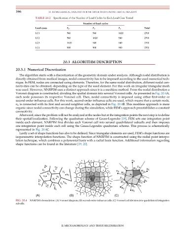
was used. However, NNRPIM uses a distinct approach since it is a meshless method. From the nodal distribution a
Voronoï diagram is constructed, dividing the spatial domain into several Voronoï cells. As presented in Fig. 20.4A,
each node possesses its respective Voronoï cell. Then, nodal connectivity is imposed using either first-order or
second-order influence cells. For this work, second-order influence cells are used, which means that a certain node,
n i , is connected with its first and second neighbor cells, as depicted in Fig. 20.4B. This meshless approach is more
organic since nodal connectivity can change during the simulation, while FEM’sapproachpreestablishesaconstant
connectivity.
Afterward, since the problem will not be analyzed at the nodes but at the integration points the next step is to define
their spatial localization. Following the quadrature scheme of Gauss-Legendre [19], FEM sets one integration point
inside each element. NNRPIM first divides each Voronoï cell into several quadrilateral subcells and then imposes
one integration point inside each cell using the Gauss-Legendre quadrature scheme. This process is schematically
represented in Fig. 20.4C.
Lastly a set of shape functions has also to be defined. Since triangular elements are used, FEM’s shape functions are
isoparametric interpolation functions. The shape function of NNRPIM is constructed using the radial point interpo-
lation technique, which combines a polynomial basis with a radial basis function. Additional information regarding
shape functions can be found in the literature [19, 20].

FIG. 20.4 NNRPIM’s formulation: (A) Voronoï diagram; (B) second-order influence cells; (C) Voronoï cell division into quadrilateral integration
subcells.

II. MECHANOBIOLOGY AND TISSUE REGENERATION