Page 397 - Advances in Biomechanics and Tissue Regeneration

394 20. BIOMECHANICAL ANALYSIS OF BONE TISSUE SURROUNDING DENTAL IMPLANTS

certain healing period, a state of equilibrium is achieved in which bone loss is minimal and implant failure rate is low.
Ideally a dental implant should have a biocompatible chemical composition to avoid adverse tissue reactions, excellent
corrosion resistance within the physiological limits, high wear resistance, and an elasticity modulus close to the bone.
In this way, bone resorption around the implant would be minimized, and stress shielding would be avoided. In this
work a standard dental implant of a titanium alloy with a conical thread is used [12].
Its impact on the trabecular morphology of the mandible is studied with the remodeling algorithm proposed in
previous works [13, 14]. With this mechanical model the adaptation and remodeling of the trabecular structure around
the implant are numerically simulated using two distinct numerical approaches—finite element method (FEM) and
Natural Neighbor Radial Point Interpolation Method (NNRPIM). To study this adaptation process, two computational
models are created. The following sections explain in detail the computational simulation conducted and the trabec-
ular morphologies obtained.

20.2 COMPUTATIONAL MODEL

This section describes the construction of a computational model of a single dental implant inserted in a patch of
mandible bone. Two distinct two-dimensional models are designed, and a set of loading conditions are applied to
reproduce the physiological loading scenario of a tooth.

20.2.1 Single Dental Implant

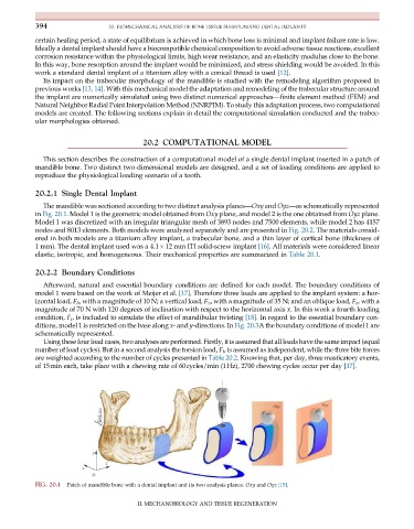
The mandible was sectioned according to two distinct analysis planes—Oxy and Oyz—as schematically represented
in Fig. 20.1. Model 1 is the geometric model obtained from Oxy plane, and model 2 is the one obtained from Oyz plane.
Model 1 was discretized with an irregular triangular mesh of 3893 nodes and 7500 elements, while model 2 has 4157
nodes and 8013 elements. Both models were analyzed separately and are presented in Fig. 20.2. The materials consid-
ered in both models are a titanium alloy implant, a trabecular bone, and a thin layer of cortical bone (thickness of
1 mm). The dental implant used was a 4.1 12 mm ITI solid-screw implant [16]. All materials were considered linear
elastic, isotropic, and homogeneous. Their mechanical properties are summarized in Table 20.1.

20.2.2 Boundary Conditions
Afterward, natural and essential boundary conditions are defined for each model. The boundary conditions of
model 1 were based on the work of Meijer et al. [17]. Therefore three loads are applied to the implant system: a hor-
izontal load, F h , with a magnitude of 10 N; a vertical load, F v , with a magnitude of 35 N; and an oblique load, F o , with a
magnitude of 70 N with 120 degrees of inclination with respect to the horizontal axis x. In this work a fourth loading
condition, F t , is included to simulate the effect of mandibular twisting [18]. In regard to the essential boundary con-
ditions, model 1 is restricted on the base along x- and y-directions. In Fig. 20.3A the boundary conditions of model 1 are
schematically represented.
Using these four load cases, two analyses are performed. Firstly, it is assumed that all loads have the same impact (equal
number of load cycles). But in a second analysis the torsion load, F t , is assumed as independent, while the three bite forces
are weighted according to the number of cycles presented in Table 20.2. Knowing that, per day, three masticatory events,
of 15min each, take place with a chewing rate of 60cycles/min (1Hz), 2700 chewing cycles occur per day [17].

FIG. 20.1 Patch of mandible bone with a dental implant and its two analysis planes: Oxy and Oyz [15].

II. MECHANOBIOLOGY AND TISSUE REGENERATION