Page 400 - Advances in Biomechanics and Tissue Regeneration

20.3 ALGORITHM DESCRIPTION 397

20.3.2 Mechanical Analysis
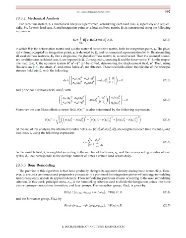
For each time instant, t j , a mechanical analysis is performed, considering each load case, k, separately and sequen-
tially. So, for each load case, k, and integration point, x I , a local stiffness matrix, K I , is constructed using the following
expression:

Z
T
T
K I5 B c I B I dΩ I 5^ w I B c I B I (20.1)
I
I
Ω I
in which B I is the deformation matrix and c I is the material constitutive matrix, both for integration point, x I . The phys-
ical volume occupied by integration point, x I , is denoted by Ω I and its numerical representation by ^ w I . By assembling
all local stiffness matrices, K I , into a single one, the global stiffness matrix, K, is constructed. Then the essential bound-
k
ary conditions for each load case, k, are imposed in K. Consequently, knowing K and the force vector, f , for the respec-
k
k
k
k
tive load case, k, the equation system K u ¼f can be solved, determining the displacement field, u . Then, using
k
k
Hooke’s law [13], the strain, ε , and stress fields, σ , are obtained. These two fields allow the calculus of the principal
k
stresses field, σ(x I ) i , with the following:
" # !
k k
σ xx x I ðÞ k 10
ðÞ σ xy x I
det k k σ x I i ¼ 0 (20.2)
ðÞ
ðÞ σ yy x I
σ xy x I ðÞ 01
k
and principal directions field, n(x I ) i , with
" # !( k )
k k
ðÞ σ xy x I
σ xx x I ðÞ k 10 n x x I i
ðÞ
k k σ x I i k ¼ 0 (20.3)
ðÞ
ðÞ σ yy x I
σ xy x I ðÞ 01 n y x I i
ðÞ
k
Moreover the von Mises effective stress field, σ x I , is also determined by the following expression:
ðÞ
s ffiffiffiffiffiffiffiffiffiffiffiffiffiffiffiffiffiffiffiffiffiffiffiffiffiffiffiffiffiffiffiffiffiffiffiffiffiffiffiffiffiffiffiffiffiffiffiffiffiffiffiffiffiffiffiffiffiffiffiffiffiffiffiffiffiffiffiffiffiffiffiffiffiffiffiffiffiffiffiffiffiffiffiffiffiffiffiffiffiffiffiffiffiffiffiffiffiffiffiffiffiffiffiffiffiffiffiffiffiffiffiffiffiffiffiffiffiffiffiffiffiffiffiffiffiffiffiffiffiffi
1 2 2 2

k k k k k k k
σ x I σ x I 1 ðÞ + σ x I 2 ðÞ + σ x I 3 ðÞ (20.4)
ðÞ σ x I 1
ðÞ σ x I 3
ðÞ σ x I 2
ðÞ ¼
2
k
k
k
k
k
At the end of this analysis, the obtained variable fields, λ¼{u j ,ε j ,σ j ,σ(n) j ,n j }, are weighted at each time instant, t j , and
load case, k, using the following expression:
d k λ
n k k
X
(20.5)
X
n k
λ ¼
k¼1 d k
k¼1
So the variable field, λ, is weighted according to the number of load cases, n k , and the corresponding number of load
cycles, d k , that corresponds to the average number of times a certain load occurs daily.
20.3.3 Bone Remodeling
The premise of this algorithm is that bone gradually changes its apparent density during bone remodeling. How-
ever, to ensure a continuous and progressive process, only a portion of the integration points will undergo remodeling
and consequently update its apparent density. These remodeling points are chosen according to the used remodeling
criterion. In this work, principal stress, σ 11 , is the remodeling criterion used to divide the integration points into three
distinct groups—resorption, formation, and lazy groups. The resorption group, R(x I ), is given by.
(20.6)
R x I 2 σ 11min ,σ 11min + α 4σ 11 , 8R x I 2 ℝ½½ ðÞ
ðÞ
and the formation group, F(x I ), by
F x I 2Šσ 11max β 4σ 11 ,σ 11max Š, 8F x I 2 ℝ (20.7)
ðÞ
ðÞ
II. MECHANOBIOLOGY AND TISSUE REGENERATION