Page 410 - Aircraft Stuctures for Engineering Student

10.3 Wings 391

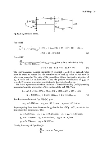
Fig. 10.25 qb distribution (N/mm).

For cell I1

+95.5 x 68 - 69 x 571
For cell I11

+45.5 x 202 - 95.5 x 68 - 95.5 x 1061 (VI
The solely numerical terms in Eqs (iii) to (v) represent fR qb(ds/t) for each cell. Care
must be taken to ensure that the contribution of each qb value to this term is
interpreted correctly. The path of the integration follows the positive direction of
qS,o in each cell, i.e. anticlockwise. Thus, the positive contribution of qb,83 to
fI qb(ds/t) becomes a negative contribution to fII qb(ds/r) and so on.
The fourth equation required for a solution is obtained from Eq. (10.30) by taking
moments about the intersection of the x axis and the web 572. Thus

0 = -69.0 x 250 x 1270 - 69.0 x 150 x 1270 + 45.5 x 330 x 1020
+2 x 265 OOOqS,o,I + 2 x 213 OOOqS,o,II + 2 x 413 OOOqS,o,III (vi>
Simultaneous solution of Eqs (iii)-(vi) gives

qs:o,r = 5.5 N/mm! 4S,O,II = 10.2 N/-, %,O:III = 16.5 N/=
Superimposing these shear flows on the qb distribution of Fig. 10.25, we obtain the
final shear flow distribution. Thus

q34 5.5N/m~1. q23 = @7 10.2N/=, q12 = q56 16.5N/mm
g61 = 62.0 N/mm, q57 = 79.0 N/mm, q72 = 89.2 N/mm

q48 74.5N/1nm, q83 = 64.3N/mm
Finally, from any of Eqs (iii)-(v)
de
- = 1.16 x 10-6rad/mm
dz